I Solutions ch. 10 - Clustering

Solutions to exercises of chapter 10.

I.1 Exercise 1

First we need to read the image data and transform it into a suitable format for analysis:

library(EBImage)
library(ggplot2)


img <- readImage("data/histology/Emphysema_H_and_E.jpg")

imgDim <- dim(img)

imgDF <- data.frame(
  x = rep(1:imgDim[1], imgDim[2]),
  y = rep(imgDim[2]:1, each=imgDim[1]),
  r = as.vector(img[,,1]),
  g = as.vector(img[,,2]),
  b = as.vector(img[,,3])
)

Next we will perform kmeans clustering for k in the range 1:9. This is computationally quite intensive, so we’ll use parallel processing:

library(doMC)

## Loading required package: foreach

## Loading required package: iterators

## Loading required package: parallel

registerDoMC()
k=1:9
set.seed(42)
res <- foreach(
  i=k, 
  .options.multicore=list(set.seed=FALSE)) %dopar% kmeans(imgDF[,c("r", "g", "b")], i, nstart=50)

We can now plot total within-cluster sum of squares against k:

plot_tot_withinss <- function(kmeans_output){
  tot_withinss <- sapply(k, function(i){kmeans_output[[i]]$tot.withinss})
  qplot(k, tot_withinss, geom=c("point", "line"), 
        ylab="Total within-cluster sum of squares") + theme_bw()
}

plot_tot_withinss(res)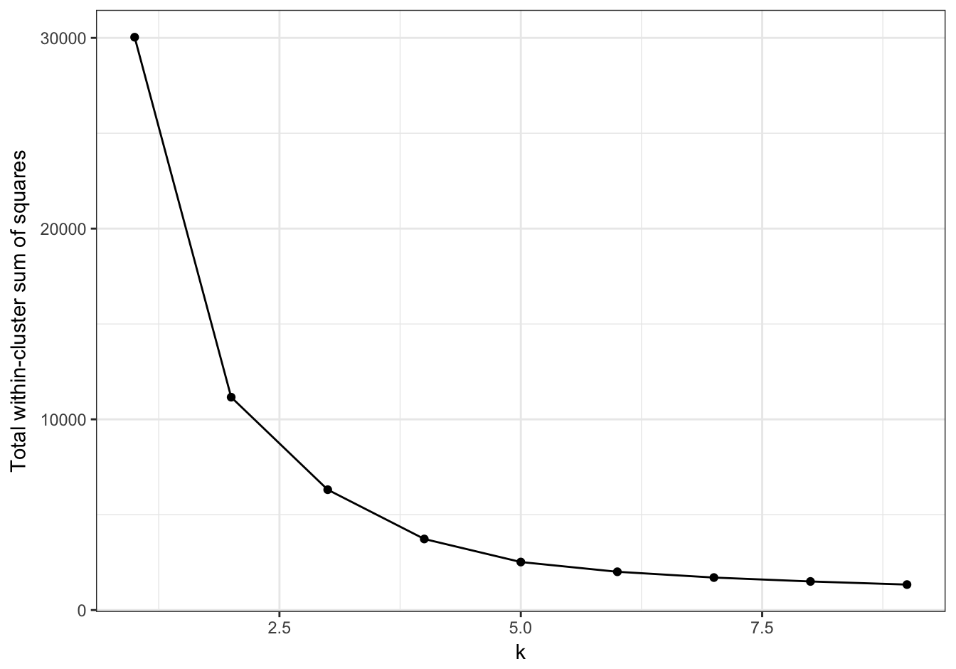

Figure I.1: Variance within the clusters of pixels. Total within-cluster sum of squares plotted against k.

The plot of total within-cluster sum of squares against k (figure I.1) shows an elbow at k=2, indicating that most of the variance in the image can be described by just two clusters. Let’s plot the clusters for k=2.

clusterColours <- rgb(res[[2]]$centers) 
ggplot(data = imgDF, aes(x = x, y = y)) + 
  geom_point(colour = clusterColours[res[[2]]$cluster]) +
  xlab("x") +
  ylab("y") +
  theme_minimal()

Figure I.2: Result of k-means clustering of pixels based on colour for k=2.

Segmentation of the image with k=2 separates air-spaces from all other objects (figure I.2). Therefore, the difference in pixel colour between the air-spaces and other objects accounts for most of the variance in the data-set (image).

Let’s now take a look at a segmentation of the image using k=4.

clusterColours <- rgb(res[[4]]$centers) 
ggplot(data = imgDF, aes(x = x, y = y)) + 
  geom_point(colour = clusterColours[res[[4]]$cluster]) +
  xlab("x") +
  ylab("y") +
  theme_minimal()

Figure I.3: Result of k-means clustering of pixels based on colour for k=4.

K-means clustering with k=4 rapidly and effectively segments the image of the histological section into the biological objects we can see by eye. A manual segmentation of the same image would be very laborious. This exercise highlights the importance of

N.B. the cluster centres provide the mean pixel intensities for the red, green and blue channels and we have used this information to colour the pixels belonging to each cluster (figure I.3).