D Solutions ch. 5 - Nearest neighbours
Solutions to exercises of chapter 5.
D.1 Exercise 1
Load libraries
library(caret)## Loading required package: lattice## Loading required package: ggplot2library(RColorBrewer)
library(doMC)## Loading required package: foreach## Loading required package: iterators## Loading required package: parallellibrary(corrplot)Prepare for parallel processing
registerDoMC()Load data
load("data/wheat_seeds/wheat_seeds.Rda")Partition data
set.seed(42)
trainIndex <- createDataPartition(y=variety, times=1, p=0.7, list=F)
varietyTrain <- variety[trainIndex]
morphTrain <- morphometrics[trainIndex,]
varietyTest <- variety[-trainIndex]
morphTest <- morphometrics[-trainIndex,]

summary(varietyTrain)
## Canadian Kama Rosa
## 49 49 49summary(varietyTest)## Canadian Kama Rosa
## 21 21 21Data check: zero and near-zero predictors
nzv <- nearZeroVar(morphTrain, saveMetrics=T)
nzv
## freqRatio percentUnique zeroVar nzv
## area 1.5 93.87755 FALSE FALSE
## perimeter 1.0 85.03401 FALSE FALSE
## compactness 1.0 93.19728 FALSE FALSE
## kernLength 1.5 91.83673 FALSE FALSE
## kernWidth 1.5 91.15646 FALSE FALSE
## asymCoef 1.0 98.63946 FALSE FALSE
## grooveLength 1.0 77.55102 FALSE FALSEData check: are all predictors on same scale?
summary(morphTrain)## area perimeter compactness kernLength
## Min. :10.74 Min. :12.57 Min. :0.8081 Min. :4.902
## 1st Qu.:12.28 1st Qu.:13.46 1st Qu.:0.8571 1st Qu.:5.253
## Median :14.29 Median :14.28 Median :0.8735 Median :5.504
## Mean :14.86 Mean :14.56 Mean :0.8712 Mean :5.632
## 3rd Qu.:17.45 3rd Qu.:15.74 3rd Qu.:0.8880 3rd Qu.:5.979
## Max. :21.18 Max. :17.25 Max. :0.9108 Max. :6.675
## kernWidth asymCoef grooveLength
## Min. :2.630 Min. :0.7651 Min. :4.605
## 1st Qu.:2.947 1st Qu.:2.5965 1st Qu.:5.028
## Median :3.212 Median :3.5970 Median :5.222
## Mean :3.258 Mean :3.6679 Mean :5.406
## 3rd Qu.:3.563 3rd Qu.:4.6735 3rd Qu.:5.878
## Max. :4.033 Max. :8.4560 Max. :6.550featurePlot(x = morphTrain,
y = varietyTrain,
plot = "box",
## Pass in options to bwplot()
scales = list(y = list(relation="free"),
x = list(rot = 90)),
layout = c(3,3))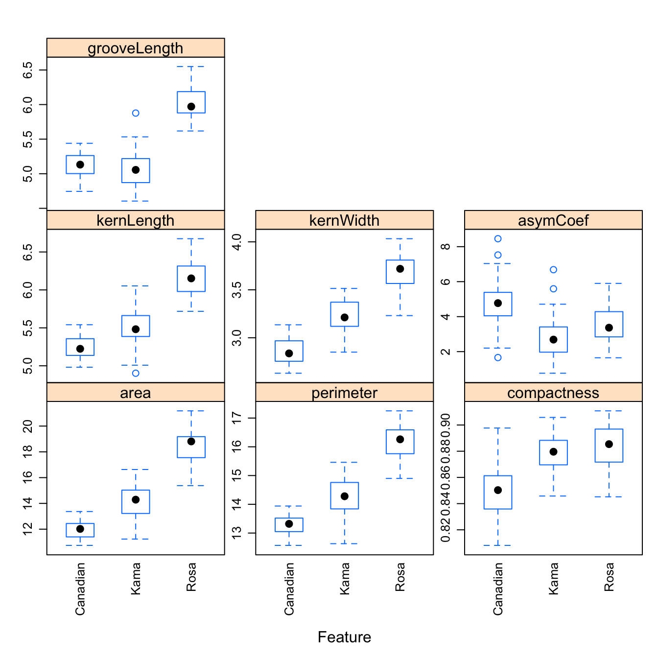
Figure D.1: Boxplots of the 7 geometric parameters in the wheat data set
Data check: pairwise correlations between predictors
corMat <- cor(morphTrain)
corrplot(corMat, order="hclust", tl.cex=1)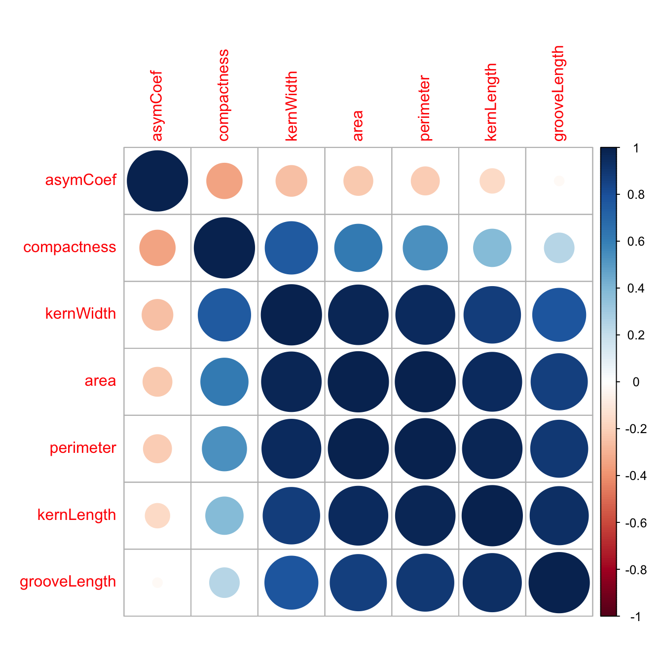
Figure D.2: Correlogram of the wheat seed data set.
highCorr <- findCorrelation(corMat, cutoff=0.75)
length(highCorr)
## [1] 4names(morphTrain)[highCorr]## [1] "area" "kernWidth" "perimeter" "kernLength"Data check: skewness
featurePlot(x = morphTrain,
            y = varietyTrain,
            plot = "density",
            ## Pass in options to xyplot() to
            ## make it prettier
            scales = list(x = list(relation="free"),
                          y = list(relation="free")),
            adjust = 1.5,
            pch = "|",
            layout = c(3, 3),
            auto.key = list(columns = 3))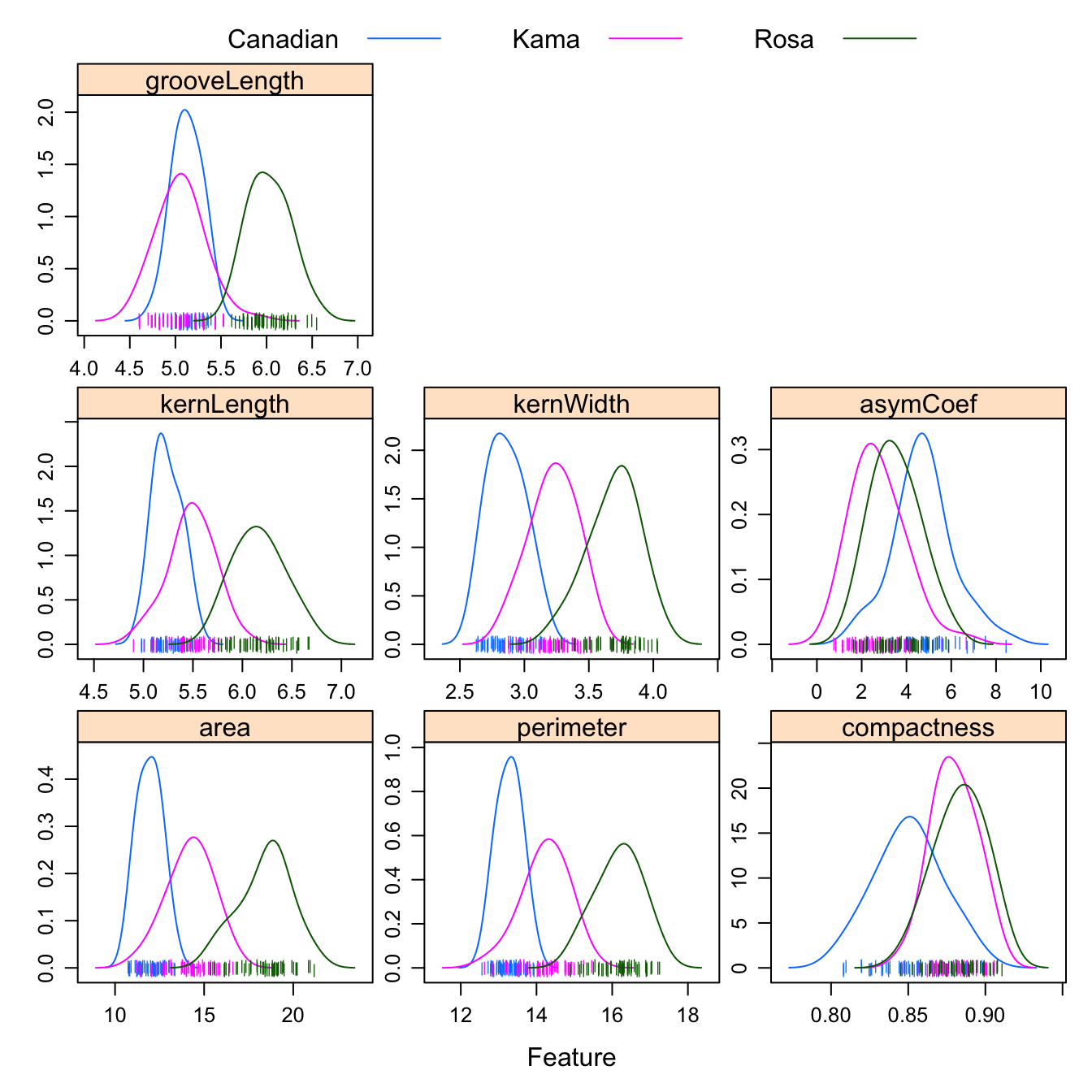
Figure D.3: Density plots of the 7 geometric parameters in the wheat data set
Create a ‘grid’ of values of k for evaluation:
tuneParam <- data.frame(k=seq(1,50,2))Generate a list of seeds for reproducibility (optional) based on grid size
set.seed(42)
seeds <- vector(mode = "list", length = 101)
for(i in 1:100) seeds[[i]] <- sample.int(1000, length(tuneParam$k))
seeds[[101]] <- sample.int(1000,1)
Set training parameters. In the example in chapter 5 pre-processing was performed outside the cross-validation process to save time for the purposes of the demonstration. Here we have a relatively small data set, so we can do pre-processing within each iteration of the cross-validation process. We specify the option preProcOptions=list(cutoff=0.75) to set a value for the pairwise correlation coefficient cutoff.
train_ctrl <- trainControl(method="repeatedcv",
                   number = 10,
                   repeats = 10,
                   preProcOptions=list(cutoff=0.75),
                   seeds = seeds)
Run training
knnFit <- train(morphTrain, varietyTrain,
                method="knn",
                preProcess = c("center", "scale", "corr"),
                tuneGrid=tuneParam,
                trControl=train_ctrl)
knnFit
## k-Nearest Neighbors
##
## 147 samples
## 7 predictor
## 3 classes: 'Canadian', 'Kama', 'Rosa'
##
## Pre-processing: centered (3), scaled (3), remove (4)
## Resampling: Cross-Validated (10 fold, repeated 10 times)
## Summary of sample sizes: 133, 132, 132, 132, 132, 132, ...
## Resampling results across tuning parameters:
##
## k Accuracy Kappa
## 1 0.8429963 0.7644190
## 3 0.9060916 0.8591664
## 5 0.8809414 0.8214171
## 7 0.8764249 0.8145913
## 9 0.8840989 0.8260932
## 11 0.8900989 0.8350932
## 13 0.8974799 0.8461701
## 15 0.8981465 0.8471701
## 17 0.8981465 0.8471701
## 19 0.8941465 0.8411868
## 21 0.8955751 0.8433490
## 23 0.8934322 0.8400932
## 25 0.8920989 0.8381099
## 27 0.8921465 0.8381868
## 29 0.8928132 0.8391868
## 31 0.8907656 0.8360598
## 33 0.8893370 0.8339060
## 35 0.8819560 0.8228372
## 37 0.8813370 0.8219221
## 39 0.8853370 0.8279221
## 41 0.8880513 0.8319908
## 43 0.8893846 0.8339908
## 45 0.8921465 0.8381614
## 47 0.8934799 0.8401614
## 49 0.8920513 0.8379992
##
## Accuracy was used to select the optimal model using the largest value.
## The final value used for the model was k = 3.Plot cross validation accuracy as a function of k
plot(knnFit)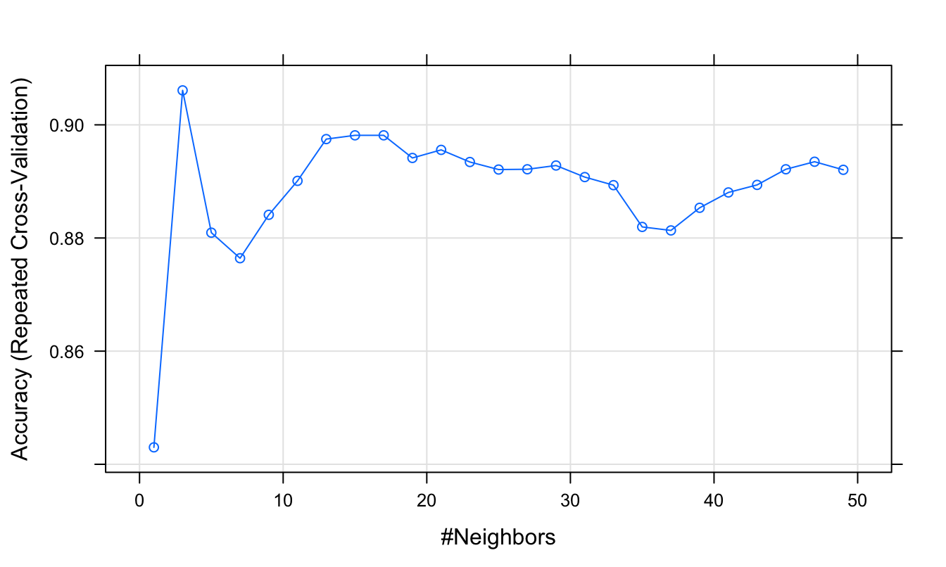
Figure D.4: Accuracy (repeated cross-validation) as a function of neighbourhood size for the wheat seeds data set.
Predict the class (wheat variety) of the observations in the test set.
test_pred <- predict(knnFit, morphTest)
confusionMatrix(test_pred, varietyTest)
## Confusion Matrix and Statistics
##
## Reference
## Prediction Canadian Kama Rosa
## Canadian 18 4 0
## Kama 3 16 2
## Rosa 0 1 19
##
## Overall Statistics
##
## Accuracy : 0.8413
## 95% CI : (0.7274, 0.9212)
## No Information Rate : 0.3333
## P-Value [Acc > NIR] : < 2.2e-16
##
## Kappa : 0.7619
## Mcnemar's Test P-Value : NA
##
## Statistics by Class:
##
## Class: Canadian Class: Kama Class: Rosa
## Sensitivity 0.8571 0.7619 0.9048
## Specificity 0.9048 0.8810 0.9762
## Pos Pred Value 0.8182 0.7619 0.9500
## Neg Pred Value 0.9268 0.8810 0.9535
## Prevalence 0.3333 0.3333 0.3333
## Detection Rate 0.2857 0.2540 0.3016
## Detection Prevalence 0.3492 0.3333 0.3175
## Balanced Accuracy 0.8810 0.8214 0.9405