13 Deep Learning
13.1 Multilayer Neural Networks
Neural networks with multiple layers are increasingly used to attack a variety of complex problems under the umberella of deep learning (Angermueller and Stegle 2016).
In this final section we will explore the basics of deep learning for image classification using a set of images taken from the animated TV series Rick and Morty. For those unfamiliar with Rick and Morty, the series revolves around the adventures of Rick Sanchez, an alcoholic, arguably sociopathic scientist, and his neurotic grandson, Morty Smith. Although many scientists aspire to be like Rick, they’re usually more like a Jerry.
Our motivating goal in this section is to develop an image classification algorithm capable of telling us whether any given image contains Rick or not: a binary classification task with two classes, Rick or not Rick. For training purposes we have downloaded several thousand random images of Rick and several thousand images without Rick from the website Master of All Science.
13.1.1 Reading in images
As with any machine learning application, it’s important to both have some question in mind (in this case “can we identify images that contain Rick Sanchez”), and understand the dataset(s) we’re using.
The image data can be found in the directory {data/RickandMorty/data/}. We begin by loading in some images of Rick using the {readJPEG} and {grid.raster} functions.
library(jpeg)
library(grid)
set.seed(12345) #Set random number generator for the session
im <- readJPEG("data/RickandMorty/data/AllRickImages/Rick_1.jpg")
grid.raster(im, interpolate=FALSE)
Let’s understand take a closer look at this dataset. We can use the funciton {dim(im)} to return the image dimensions. In this case each image is stored as a jpeg file, with \(90 \times 160\) pixel resolution and \(3\) colour channels (RGB). This loads into R as \(160 \times 90 \times 3\) array. We could start by converting the image to grey scale, reducing the dimensions of the input data. However, each channel will potentially carry novel information, so ideally we wish to retain all of the information. You can take a look at what information is present in the different channels by plotting them individually using e.g., {grid.raster(im[,,3], interpolate=FALSE)}. Whilst the difference is not so obvious here, we can imagine sitations where different channels could be dramamtically different, for example, when dealing with remote observation data from satellites, where we might have visible wavelength alongside infrared and a variety of other spectral channels.
Since we plan to retain the channel information, our input data is a tensor of dimension \(90 \times 160 \times 3\) i.e., height x width x channels. Note that this ordering is important, as the the package we’re using expects this ordering (be careful, as other packages can expect a different ordering).
Before building a neural network we first have to load the data and construct a training, validation, and test set of data. Whilst the package we’re using has the ability to specify this on the fly, I prefer to manually seperate out training/test/validation sets, as it makes it easier to later debug when things go wrong.
First load all Rick images and all not Rick images from their directory. We can get a list of all the Rick and not Rick images using {list.files}:
files1 <- list.files(path = "data/RickandMorty/data/AllRickImages/", pattern = "jpg")
files2 <- list.files(path = "data/RickandMorty/data/AllMortyImages/", pattern = "jpg")
After loading the lsit of files we can see we have \(2211\) images of Rick and \(3046\) images of not Rick. Whilst this is a slightly unbiased dataset it is not dramatically so; in cases where there is extreme inbalance in the number of class observations we may have to do something extra, such as data augmentation, or assinging weights during training.
We next preallocate an empty array to store these training images for the Rick and not Rick images (an array of dimension \(5257 \times 90 \times 160 \times 3\)):
allX <- array(0, dim=c(length(files1)+length(files2),dim(im)[1],dim(im)[2],dim(im)[3]))We can load images using the {readJPEG} function:
for (i in 1:length(files1)){
  allX[i,1:dim(im)[1],1:dim(im)[2],1:dim(im)[3]] <- readJPEG(paste("data/RickandMorty/data/AllRickImages/", files1[i], sep=""))
}
Similarly, we can load the not Rick images and store in the same array:
for (i in 1:length(files2)){
  allX[i+length(files1),1:dim(im)[1],1:dim(im)[2],1:dim(im)[3]] <- readJPEG(paste("data/RickandMorty/data/AllMortyImages/", files2[i], sep=""))
}
Next we can construct a vector of length \(5257\) containing the classification for each of the images e.g., a \(0\) if the image is a Rick and \(1\) if it is not Rick. This is simple enough using the function {rbind}, as we know the first \(2211\) images were Rick and the second lot of images are not Rick. Since we are dealing with a classification algorithm, we next convert the data to binary categorical output (that is, a Rick is now represented as \([1, 0]\) and a not Rick is a \([0, 1]\)), which we can do using the {to_categorical} conversion function:
library(kerasR)## successfully loaded keraslabels <- rbind(matrix(0, length(files1), 1), matrix(1, length(files2), 1))
allY <- to_categorical(labels, num_classes = 2)Obviously in the snippet of code above we have \(2\) classes; we could just as easily perform classificaiton with more than \(2\) classes, for example if we wanted to classify Ricky, Morty, or Jerry, and so forth.
We must now split our data in training sets, validation sets, and test sets. In fact I have already stored some seperate “test” set images in another folder that we will load in at the end, so here we only need to seperate images into training and validation sets. It’s important to note that we shouldn’t simply take the first \(N\) images for training with the remainder used for validation/testing, since this may introduce artefacts. For example, here we’ve loaded in all the Rick images in first, with the not Rick images loaded in second: if we took, say, the first \(2000\) images for training, we would be training with only Rick images, which makes our task impossible, and our algorithm will fail catastrophically.
Although there are more elegant ways to shuffle data using {caret}, here we are going to manually randomly permute the data, and then take the first \(4000\) permuted images for training, with the remainder for validation (Note: it’s crucial to permute the \(Y\) data in the same way).
vecInd <- seq(0,length(files1)+length(files2)) #A vector of indexes
trainInd <- sample(vecInd)[1:4001] #Permute and take first 4000 training
valInd <- setdiff(vecInd,trainInd) #The remainder are for val/testing

trainX <- allX[trainInd, , , ]
trainY <- allY[trainInd, 1]

valX <- allX[valInd, , , ]
valY <- allY[valInd, 1]
We are almost ready to begin building our neural networks. First can try a few things to make sure out data has been processed correctly. For example, try manually plotting several of the images and seeing if the labels are correct. Manually print out the image matrix (not a visualisation of it): think about the range of the data, and whether it will need normalising. Finally we can check to see how many of each class is in the training and validation datasets. In this case there are \(1706\) images of Rick and \(2294\) images of not Rick in the training dataset. Again, whilst there is some slight class inbalance it is not terrible, so we don’t need to perform data augmentation or assign weights to the different classes during training.
13.1.2 Constructing layers in kerasR
A user friendly package for neural networks is available via keras, an application programming interface (API) written in Python, which uses either theano or tensorflow as a back-end. An R interface for keras is available in the form of kerasR.
Before we can use kerasR we first need to load the kerasR library in R (we also need to install keras and either theano and tensorflow).
And so we come to specifying the model itself. Keras has an simple and intuitive way of specifying layers of a neural network, and kerasR makes good use of this. We first initialie the model:
mod <- Sequential()This tells keras that we’re using the Sequential API i.e., a network with the first layer connected to the second, the second to the third and so forth, which distinguishes it from more complex networks possible using the Model API. Once we’ve specified a sequential model, we have to stard adding layers to the neural network.
A standard layer of neurons can be specified using the {Dense} command; the first layer of our network must also include the dimension of the input. So, for example, if our input data was a vector of dimension \(1 \times 40\), we could add an input layer via:
mod$add(Dense(100, input_shape = c(1,40)))We also need to specfy the activation function to the next level. This can be done via {Activation()}, so our snippet of code using a Rectified Linear Unit (relu) activation would look something like:
mod$add(Dense(100, input_shape = c(1,40)))
mod$add(Activation("relu"))
This is all we need to specify a single layer of the neural network. We could add another layer of 120 neurons via:
mod$add(Dense(120))
mod$add(Activation("relu"))
Finally, we should add the output neurons. The number of output neurons will differ, but will by and large match the size of the output we’re aiming to predict. In this case we have two outputs, so will have a {Dense(2)} output. The final activation function also depends on our data. If, for example, we’re doing regression, we don’t need a final activaition (or can explicitly speify a linear activation). For a categorical outpur for one-hot data we could specify a {softmax} activation. Here we will specify a {sigmoid} activation function. Our final model would look like:
mod$add(Dense(100, input_shape = c(1,40)))
mod$add(Activation("relu"))
mod$add(Dense(120))
mod$add(Activation("relu"))
mod$add(Dense(2))
mod$add(Activation("sigmoid"))
That’s it. Simple!
13.1.3 Rick and Morty classifier using Deep Learning
Let us return to our example of image classification. Our data is slightly different to the usual inputs we’ve been dealing with: that is, we’re not dealing with an input vector, but instead have an array. In this case each image is a \(90 \times 160 \time 3\) array. So for our first layer we first have to flatten this down using {Flatten()}:
mod$add(Flatten(input_shape = c(90, 160, 3)))This should turn our \(90 \times \160 \times 3\) input into a \(1 \times 43200\) node input. We now add an intermediate layer containing \(100\) neurons, connected to the input layer with rectified linear units ({relu}):
mod$add(Activation("relu"))
mod$add(Dense(100))
Finally we connect this layer over the final output layer (two neurons) with sigmoid activation: activation
mod$add(Activation("relu"))
mod$add(Dense(2))
mod$add(Activation("sigmoid"))
The complete model should look something like:
mod <- Sequential()
mod$add(Flatten(input_shape = c(90, 160, 3)))
mod$add(Activation("relu"))
mod$add(Dense(100))
mod$add(Activation("relu"))
mod$add(Dense(1))
mod$add(Activation("sigmoid"))
We can visualise this model using the {plot_model} function (Figure 13.1).
plot_model(mod,'images/DNN1.png')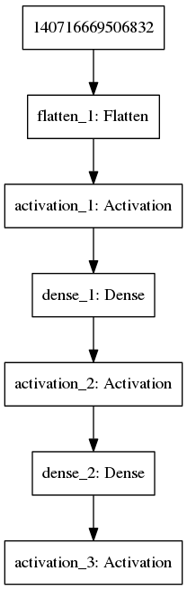
Figure 13.1: Example of a multilayer convolutional neural network
We can also print a summary of the network, for example to see how many parameters it has, using the {summary} function:
summary(mod)## <keras.engine.sequential.Sequential>In this case we see a total of \(4,320,302\) parameters. That’s a lot of parameters to tune, and not much data!
Next we need to compile and run the model. In this case we need to specify three things:
A loss function, which specifies the objective function that the model will try to minimise. A number of existing loss functions are built into keras, including the mean squared error (mean_squared_error), which is used for regression, and categorical cross entropy (categorical_crossentropy), which is used for cateogrical classification. Since we are dealing with binary classification, we will use binary cross entropy (binary_crossentropy).
An optimiser, which determines how the loss function is optimised. Possible examples include stochastic gradient descent ({SGD()}) and Root Mean Square Propagation ({RMSprop()}).
A list of metrics to return. These are additional summary statistics that keras evaluates and prints. For classification, a good choice would be accuracy (or {binary_accuracy}).
We can compile our model using {keras_compile}:
keras_compile(mod, loss = 'binary_crossentropy', metrics = c('binary_accuracy'), optimizer = RMSprop())Finally the model can be fitted to the data. When doing so we additionally need to specify the validation set (if we have one), the batch size and the number of epochs, where an epoch is one forward pass and one backward pass of all the training examples and the batch size is the number of training examples in one forward/backward pass. You may want to go and get a tea whilst this is running!
set.seed(12345)
keras_fit(mod, trainX, trainY, validation_data = list(valX, valY), batch_size = 32, epochs = 25, verbose = 1)
For this model we achieved an accuracy of \(0.5725\) on the validation dataset at epoch \(2\) (which had a corresponding accuracy of \(0.5816\) on the training set). Not great is an understatement. In fact, if we consider the inbalance in the number of classes, a niave algorithm that always asigns the data to not Rick would achieve an accuracy of \(0.57\) and \(0.60\) in the training and validation sets respectively. Another striking observation is that the accuracy itself doesn’t appear to be changing during training: a possible sign that something is amiss.
Let’s try adding in another layer to the network. Before we do so, another important point to note is that the model we have at the end of training is the one one we generated during the latest epoch, and not the model that gives the best validation accuracy. Since our aim is to have the best predictive model we will also have to introduce a callback.
In the snippet of code, below, we contruct a new network, with an additional layer containing \(70\) neurons, and introduce a callback that returns the best model at the end of our training:
mod <- Sequential()
mod$add(Flatten(input_shape = c(90, 160, 3)))
mod$add(Activation("relu"))
mod$add(Dense(100))
mod$add(Activation("relu"))
mod$add(Dense(70))
mod$add(Activation("relu"))
mod$add(Dense(1))
mod$add(Activation("sigmoid"))

callbacks <- list(ModelCheckpoint('data/RickandMorty/data/models/model.h5', monitor = "val_binary_accuracy", verbose = 0, save_best_only = TRUE, save_weights_only = FALSE, mode = "auto",period = 1))

keras_compile(mod,  loss = 'binary_crossentropy', metrics = c('binary_accuracy'), optimizer = RMSprop())

set.seed(12345)
keras_fit(mod, trainX, trainY, validation_data = list(valX, valY), batch_size = 32, epochs = 25, callbacks = callbacks, verbose = 1)
We can again visualise the model:
plot_model(mod,'images/DNN2.png')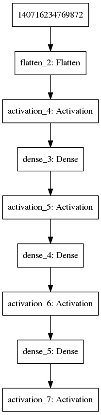
Figure 13.2: Example of a multilayer convolutional neural network
We get now get a validation accuracy of \(0.57\) with corresponding training accuracy of \(0.58\). We could try adding in extra layers, but it seems like we’re getting nowhere fast, and will need to change tactic.
We need to think a little more about what the data actually is. In this case we’re looking at a set of images. As Rick Sanchez can appear almost anywhere in the image, there’s no reason to think that a given input node should correspond in two different images, so it’s not surprising that the network did so badly. We need something that can extract out features from the image irregardless of where Rick is. There are approaches build precicesly for image analysis that do just this: convolutional neural networks.
13.2 Convolutional neural networks
Convolutional neural networks essentially scan through an image and extract out a set of features. In multilayer neural networks, these features might then be passed on to deeper layers (other convolutional layers or standard neurons) as shown in Figure 13.3.

Figure 13.3: Example of a multilayer convolutional neural network
In kerasR we can add a convolutional layer using {Conv2D}. A multilayer convolutional neural network might look something like:
mod <- Sequential()
mod$add(Conv2D(filters = 20, kernel_size = c(5, 5),input_shape = c(90, 160, 3)))
mod$add(Activation("relu"))
mod$add(MaxPooling2D(pool_size=c(3, 3)))
mod$add(Conv2D(filters = 20, kernel_size = c(5, 5)))
mod$add(Activation("relu"))
mod$add(MaxPooling2D(pool_size=c(3, 3)))
mod$add(Conv2D(filters = 64, kernel_size = c(5, 5)))
mod$add(Activation("relu"))
mod$add(MaxPooling2D(pool_size=c(3, 3)))
mod$add(Flatten())
mod$add(Dense(100))
mod$add(Activation("relu"))
mod$add(Dropout(0.6))
mod$add(Dense(1))
mod$add(Activation("sigmoid"))

callbacks <- list(ModelCheckpoint('data/RickandMorty/data/models/convmodel.h5', monitor = "val_binary_accuracy", verbose = 0, save_best_only = TRUE, save_weights_only = FALSE, mode = "auto", period = 1))

keras_compile(mod,  loss = 'binary_crossentropy', metrics = c('binary_accuracy'), optimizer = RMSprop())
set.seed(12345)
keras_fit(mod, trainX, trainY, validation_data = list(valX, valY), batch_size = 32, epochs = 25, callbacks = callbacks, verbose = 1)
Again we can visualise this network:
plot_model(mod,'images/DNN3.png')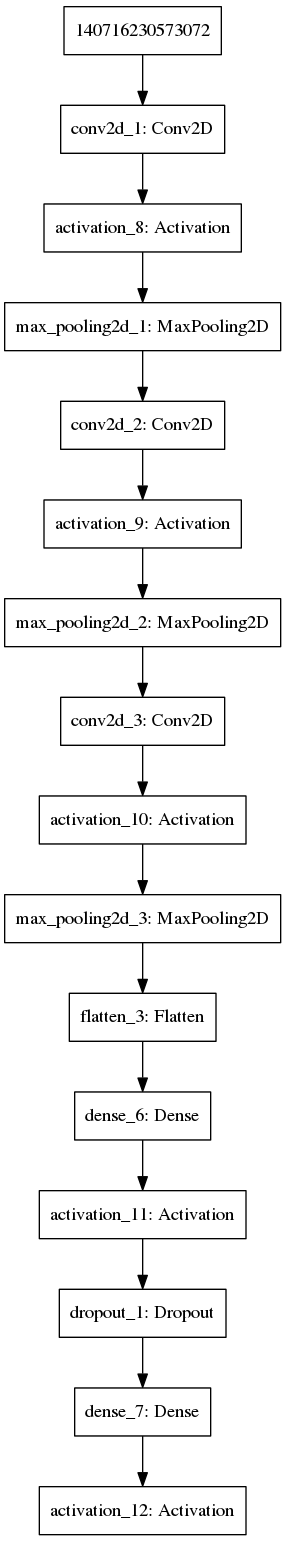
Figure 13.4: Example of a multilayer convolutional neural network
Okay, so now we have achieved a better accuracy: we have an accuracy of \(0.9196\) on the validation dataset at epoch \(24\), with a training accuracy of \(0.9838\). Whilst this is still not great, it’s accurate enough to begin useuflly making predictions and visualising the results. We have a trained model for classification of Rick, we can use it to make predictions for images not present in either the training or validation datasets. First load in the new set of images, which can be found in the {predictions} subfolder:
files <- list.files(path = "data/RickandMorty/data/predictions/",pattern = "jpg")
predictX  <- array(0,dim=c(length(files),90,160,3))
for (i in 1:length(files)){
  x <- readJPEG(paste("data/RickandMorty/data/predictions/", files[i],sep=""))
  predictX[i,1:90,1:160,1:3] <- x[1:90,1:160,1:3]
}
A hard classification can be assigned using the {keras_predict_classes} function, whilst the probability of assignment to either class can be evaluated using {keras_predict_proba} (this can be useful for images that might be ambiguous).
probY <- keras_predict_proba(mod, predictX)
predictY <- keras_predict_classes(mod, predictX)
We can plot an example:
choice = 13
dev.off()
## null device
## 1if (predictY[choice]==1) {
grid.raster(predictX[choice,1:90,1:160,1:3], interpolate=FALSE)
grid.text(label='Rick',x = 0.4, y = 0.77,just = c("left", "top"), gp=gpar(fontsize=15, col="black"))
} else {
grid.raster(predictX[choice,1:90,1:160,1:3], interpolate=FALSE)
grid.text(label='Not Rick',x = 0.4, y = 0.77,just = c("left", "top"), gp=gpar(fontsize=15, col="grey"))
}choice = 1
dev.off()## null device
## 1if (predictY[choice]==1) {
grid.raster(predictX[choice,1:90,1:160,1:3], interpolate=FALSE)
grid.text(label='Rick',x = 0.4, y = 0.77,just = c("left", "top"), gp=gpar(fontsize=15, col="black"))
} else {
grid.raster(predictX[choice,1:90,1:160,1:3], interpolate=FALSE)
grid.text(label='Not Rick',x = 0.4, y = 0.77,just = c("left", "top"), gp=gpar(fontsize=15, col="black"))
}choice = 6
dev.off()## null device
## 1if (predictY[choice]==1) {
grid.raster(predictX[choice,1:90,1:160,1:3], interpolate=FALSE)
grid.text(label='Rick',x = 0.4, y = 0.77,just = c("left", "top"), gp=gpar(fontsize=15, col="black"))
} else {
grid.raster(predictX[choice,1:90,1:160,1:3], interpolate=FALSE)
grid.text(label='Not Rick',x = 0.4, y = 0.77,just = c("left", "top"), gp=gpar(fontsize=15, col="black"))
}dev.off()## null device
## 1choice = 16
if (predictY[choice]==1) {
grid.raster(predictX[choice,1:90,1:160,1:3], interpolate=FALSE)
grid.text(label='Rick',x = 0.4, y = 0.77,just = c("left", "top"), gp=gpar(fontsize=15, col="black"))
} else {
grid.raster(predictX[choice,1:90,1:160,1:3], interpolate=FALSE)
grid.text(label='Not Rick: must be a Jerry',x = 0.2, y = 0.77,just = c("left", "top"), gp=gpar(fontsize=15, col="black"))
}13.2.1 Checking the models
Although our model seems to be doing reasonablly, it always helps to see where exactly it’s going wrong. Let’s take a look at a few of the false positives and a few of the false negatives.
probvalY <- keras_predict_proba(mod, valX)
predictvalY <- keras_predict_classes(mod, valX)

TP <- which(predictvalY==1 & valY==1)
FN <- which(predictvalY==0 & valY==1)
TN <- which(predictvalY==0 & valY==0)
FP <- which(predictvalY==1 & valY==0)
Let’s see where we go it right:
dev.off()## null device
## 1grid.raster(valX[TP[1],1:90,1:160,1:3], interpolate=FALSE, width = 0.7, x = 0.5, y=0.2)
grid.raster(valX[TP[2],1:90,1:160,1:3], interpolate=FALSE, width = 0.7, x = 0.5, y=0.5)
grid.raster(valX[TP[3],1:90,1:160,1:3], interpolate=FALSE, width = 0.7, x = 0.5, y=0.8)And wrong (false negative):
dev.off()## null device
## 1grid.raster(valX[FN[1],1:90,1:160,1:3], interpolate=FALSE, width = 0.7, x = 0.5, y=0.2)
grid.raster(valX[FN[2],1:90,1:160,1:3], interpolate=FALSE, width = 0.7, x = 0.5, y=0.5)
grid.raster(valX[FN[3],1:90,1:160,1:3], interpolate=FALSE, width = 0.7, x = 0.5, y=0.8)Or false positives:
dev.off()## null device
## 1grid.raster(valX[FP[1],1:90,1:160,1:3], interpolate=FALSE, width = 0.7, x = 0.5, y=0.2)
grid.raster(valX[FP[2],1:90,1:160,1:3], interpolate=FALSE, width = 0.7, x = 0.5, y=0.5)
grid.raster(valX[FP[4],1:90,1:160,1:3], interpolate=FALSE, width = 0.7, x = 0.5, y=0.8)It’s not entirely clear why exactly the network is failing in some of these cases. An alternative what exactly is going on is to take a look at which pixels are contributing the most to the classifier, as we have done during the lecture.
13.2.2 Data augmentation
Although we saw some imporovements in the previous section using convolutional neural networks, the end results were not particularly convincing. After all, previous applications in the recognition of handwritten digits (0-9) showed above human accuracy, see e.g., Neural Networks and Deep Learning. Our accuracy of approximately \(90\) percent is nowhere near human levels of accuracy. So where are we gong wrong?
We should, of course, start by considering the number of parameters versus the size of the training dataset. In our final model we had \(69,506\) parameters, and only a few thousand training images, so it is perhaps not surprising that our model is doing relatively poorly. In previous examples of digit recognition more than \(10,000\) images were used, whilst better known examples of deep learning for image classification make use of millions of images. Our task is also, arguably, a lot harder than digit recognition. After all, a handwritten \(0\) is relatively similar regardless of who wrote it. Rick Sanchez, on the other hand, can come in a diverse range of guises, with different postures, facial expressions, clothing, and even in pickle-Rick form. We may well need a vastly increased number of training; with more training data, we can begin to learn more robustly what features define a Rick. Whilst we could simply download more data from Master of All Science, an alternative approach is to atrificially increase our pool of training data by manipulating the images. For example, we could shear, warp or rotate some of the images in our training set; we could add noise and we could manipulate the colouring.
13.2.3 Asking more precise questions
Another way we could improve our accuracy is to ask more precise questions. In our application we have focused on what makes a Rick, and what makes a not Rick. Whilst there may be definable features for Rick, such as his hair and his white coat, the class not Rick is an amalgamation of all other characters and scenes in the series. A better approach would be to develop algorithms that classify Rick versus Morty. In this case we would need to tweak our training and validation datasets.
13.2.4 More complex networks
More complex learning algorithms can easily be built using Keras via the model class API rather than the sequential API. This allows, for example, learning from multiple inputs and/or outputs, with more interconnection between the different layers. We might, for example, want to include additional contextual information about the image that could serve to augment the predictions.
Another approach is to use transfer learning. This is where we make use of existing neural networks to make predictions on our specific datasets, usually fixing the top layers in place and fine tuning the lower layers to our dataset. For example, for image recognition we could make use of top perfoming neural networks on the ImageNet database. Whilst none of these networks would have been designed to identify Rick they would have been trained on millions of images, and the top levels would have been able to extract useful general features of an image.
13.3 Further reading
A particularly comprehensive introduction to Deep Learning can be found in the e-book Neural Networks and Deep Learning, written by Michael Nielsen.
Useful examples can also be found in the keras documentation.
Installing Python Linux Installing Python for Mac Python install via Conda
Installing Tensorflow Installing Keras
Solutions to exercises can be found in appendix ??.
K Solutions for use case 2
Angermueller, Tanel Pärnamaa, Christof, and Oliver Stegle. 2016. “Deep Learning for Computational Biology.” Molecular Systems Biology 12 (7): 878.