E Solutions ch. 6 - Support vector machines
Solutions to exercises of chapter 6.
E.1 Exercise 1
Load required libraries
library(caret)## Loading required package: lattice## Loading required package: ggplot2library(doMC)## Loading required package: foreach## Loading required package: iterators## Loading required package: parallellibrary(pROC)## Type 'citation("pROC")' for a citation.##
## Attaching package: 'pROC'## The following objects are masked from 'package:stats':
##
## cov, smooth, varlibrary(e1071)Define a radial SVM using the e1071 library
svmRadialE1071 <- list(
  label = "Support Vector Machines with Radial Kernel - e1071",
  library = "e1071",
  type = c("Regression", "Classification"),
  parameters = data.frame(parameter="cost",
                          class="numeric",
                          label="Cost"),
  grid = function (x, y, len = NULL, search = "grid")
    {
      if (search == "grid") {
        out <- expand.grid(cost = 2^((1:len) - 3))
      }
      else {
        out <- data.frame(cost = 2^runif(len, min = -5, max = 10))
      }
      out
    },
  loop=NULL,
  fit=function (x, y, wts, param, lev, last, classProbs, ...)
    {
      if (any(names(list(...)) == "probability") | is.numeric(y)) {
        out <- e1071::svm(x = as.matrix(x), y = y, kernel = "radial",
                          cost = param$cost, ...)
      }
      else {
        out <- e1071::svm(x = as.matrix(x), y = y, kernel = "radial",
                          cost = param$cost, probability = classProbs, ...)
      }
      out
    },
  predict = function (modelFit, newdata, submodels = NULL)
    {
      predict(modelFit, newdata)
    },
  prob = function (modelFit, newdata, submodels = NULL)
    {
      out <- predict(modelFit, newdata, probability = TRUE)
      attr(out, "probabilities")
    },
  predictors = function (x, ...)
    {
      out <- if (!is.null(x$terms))
        predictors.terms(x$terms)
      else x$xNames
      if (is.null(out))
        out <- names(attr(x, "scaling")$x.scale$`scaled:center`)
      if (is.null(out))
        out <- NA
      out
    },
  tags = c("Kernel Methods", "Support Vector Machines", "Regression", "Classifier", "Robust Methods"),
  levels = function(x) x$levels,
  sort = function(x)
  {
    x[order(x$cost), ]
  }
)
Setup parallel processing
registerDoMC(detectCores())
getDoParWorkers()
## [1] 8Load data
data(segmentationData)segClass <- segmentationData$ClassExtract predictors from segmentationData
segData <- segmentationData[,4:59]Partition data
set.seed(42)
trainIndex <- createDataPartition(y=segClass, times=1, p=0.5, list=F)
segDataTrain <- segData[trainIndex,]
segDataTest <- segData[-trainIndex,]
segClassTrain <- segClass[trainIndex]
segClassTest <- segClass[-trainIndex]
Set seeds for reproducibility (optional). We will be trying 9 values of the tuning parameter with 5 repeats of 10 fold cross-validation, so we need the following list of seeds.
set.seed(42)
seeds <- vector(mode = "list", length = 51)
for(i in 1:50) seeds[[i]] <- sample.int(1000, 9)
seeds[[51]] <- sample.int(1000,1)
We will pass the twoClassSummary function into model training through trainControl. Additionally we would like the model to predict class probabilities so that we can calculate the ROC curve, so we use the classProbs option.
cvCtrl <- trainControl(method = "repeatedcv",
                       repeats = 5,
                       number = 10,
                       summaryFunction = twoClassSummary,
                       classProbs = TRUE,
                       seeds=seeds)
Tune SVM over the cost parameter. The default grid of cost parameters start at 0.25 and double at each iteration. Choosing tuneLength = 9 will give us cost parameters of 0.25, 0.5, 1, 2, 4, 8, 16, 32 and 64. The train function will calculate an appropriate value of sigma (the kernel parameter) from the data.
svmTune <- train(x = segDataTrain,
                 y = segClassTrain,
                 method = svmRadialE1071,
                 tuneLength = 9,
                 preProc = c("center", "scale"),
                 metric = "ROC",
                 trControl = cvCtrl)

svmTune
## Support Vector Machines with Radial Kernel - e1071
##
## 1010 samples
## 56 predictors
## 2 classes: 'PS', 'WS'
##
## Pre-processing: centered (56), scaled (56)
## Resampling: Cross-Validated (10 fold, repeated 5 times)
## Summary of sample sizes: 909, 909, 909, 909, 909, 909, ...
## Resampling results across tuning parameters:
##
## cost ROC Sens Spec
## 0.25 0.8822479 0.8744615 0.6788889
## 0.50 0.8889402 0.8704615 0.7111111
## 1.00 0.8920256 0.8729231 0.7283333
## 2.00 0.8908291 0.8630769 0.7494444
## 4.00 0.8856239 0.8566154 0.7494444
## 8.00 0.8761282 0.8443077 0.7422222
## 16.00 0.8627265 0.8372308 0.7200000
## 32.00 0.8530769 0.8415385 0.6988889
## 64.00 0.8493846 0.8406154 0.6916667
##
## ROC was used to select the optimal model using the largest value.
## The final value used for the model was cost = 1.svmTune$finalModel##
## Call:
## svm.default(x = as.matrix(x), y = y, kernel = "radial", cost = param$cost,
## probability = classProbs)
##
##
## Parameters:
## SVM-Type: C-classification
## SVM-Kernel: radial
## cost: 1
## gamma: 0.01785714
##
## Number of Support Vectors: 531SVM accuracy profile
plot(svmTune, metric = "ROC", scales = list(x = list(log =2)))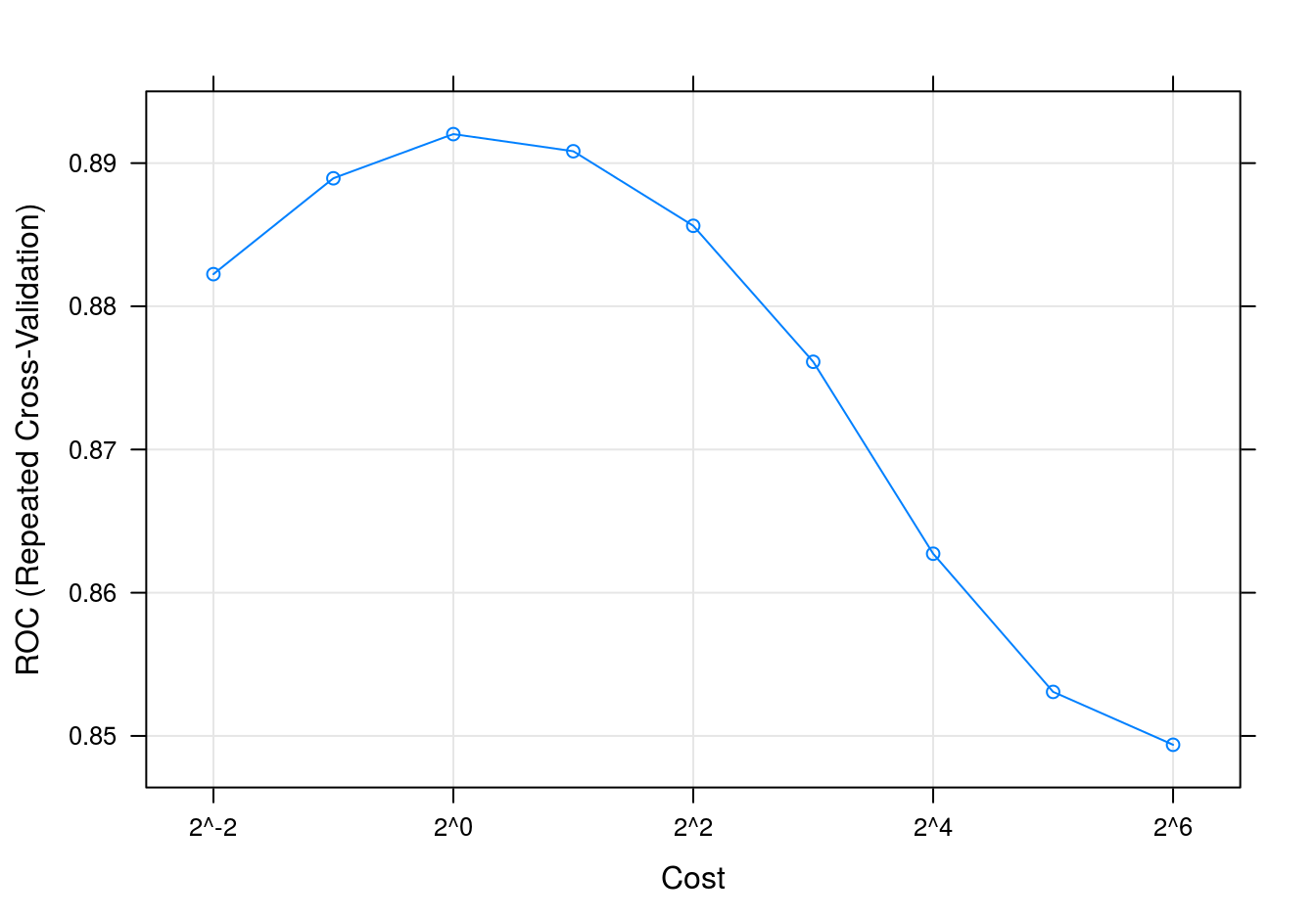
Figure E.1: SVM accuracy profile.
Test set results
#segDataTest <- predict(transformations, segDataTest)
svmPred <- predict(svmTune, segDataTest)
confusionMatrix(svmPred, segClassTest)
## Confusion Matrix and Statistics
##
## Reference
## Prediction PS WS
## PS 571 103
## WS 79 256
##
## Accuracy : 0.8196
## 95% CI : (0.7945, 0.8429)
## No Information Rate : 0.6442
## P-Value [Acc > NIR] : < 2e-16
##
## Kappa : 0.6005
## Mcnemar's Test P-Value : 0.08822
##
## Sensitivity : 0.8785
## Specificity : 0.7131
## Pos Pred Value : 0.8472
## Neg Pred Value : 0.7642
## Prevalence : 0.6442
## Detection Rate : 0.5659
## Detection Prevalence : 0.6680
## Balanced Accuracy : 0.7958
##
## 'Positive' Class : PS
## Get predicted class probabilities
svmProbs <- predict(svmTune, segDataTest, type="prob")
head(svmProbs)
## PS WS
## 3 0.2304335 0.76956646
## 5 0.9334686 0.06653138
## 9 0.7495523 0.25044774
## 10 0.8312666 0.16873341
## 13 0.9445697 0.05543032
## 14 0.7674554 0.23254457Build a ROC curve
svmROC <- roc(segClassTest, svmProbs[,"PS"])
auc(svmROC)
## Area under the curve: 0.8864Plot ROC curve.
plot(svmROC, type = "S")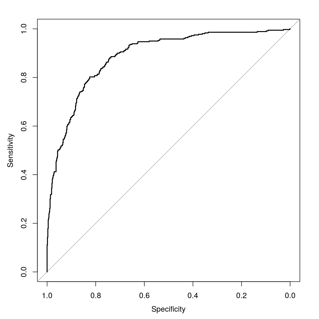
Figure E.2: SVM ROC curve for cell segmentation data set.
Calculate area under ROC curve
auc(svmROC)## Area under the curve: 0.8864