G Solutions chapter 8 - use case 1
Solutions to exercises of chapter 8.
G.1 Preparation
G.1.1 Load required libraries
library(caret)## Loading required package: lattice## Loading required package: ggplot2library(doMC)## Loading required package: foreach## Loading required package: iterators## Loading required package: parallellibrary(corrplot)## corrplot 0.84 loadedlibrary(rpart.plot)## Loading required package: rpartlibrary(pROC)## Type 'citation("pROC")' for a citation.##
## Attaching package: 'pROC'## The following objects are masked from 'package:stats':
##
## cov, smooth, varG.1.2 Define SVM model
svmRadialE1071 <- list(
  label = "Support Vector Machines with Radial Kernel - e1071",
  library = "e1071",
  type = c("Regression", "Classification"),
  parameters = data.frame(parameter="cost",
                          class="numeric",
                          label="Cost"),
  grid = function (x, y, len = NULL, search = "grid")
    {
      if (search == "grid") {
        out <- expand.grid(cost = 2^((1:len) - 3))
      }
      else {
        out <- data.frame(cost = 2^runif(len, min = -5, max = 10))
      }
      out
    },
  loop=NULL,
  fit=function (x, y, wts, param, lev, last, classProbs, ...)
    {
      if (any(names(list(...)) == "probability") | is.numeric(y)) {
        out <- e1071::svm(x = as.matrix(x), y = y, kernel = "radial",
                          cost = param$cost, ...)
      }
      else {
        out <- e1071::svm(x = as.matrix(x), y = y, kernel = "radial",
                          cost = param$cost, probability = classProbs, ...)
      }
      out
    },
  predict = function (modelFit, newdata, submodels = NULL)
    {
      predict(modelFit, newdata)
    },
  prob = function (modelFit, newdata, submodels = NULL)
    {
      out <- predict(modelFit, newdata, probability = TRUE)
      attr(out, "probabilities")
    },
  predictors = function (x, ...)
    {
      out <- if (!is.null(x$terms))
        predictors.terms(x$terms)
      else x$xNames
      if (is.null(out))
        out <- names(attr(x, "scaling")$x.scale$`scaled:center`)
      if (is.null(out))
        out <- NA
      out
    },
  tags = c("Kernel Methods", "Support Vector Machines", "Regression", "Classifier", "Robust Methods"),
  levels = function(x) x$levels,
  sort = function(x)
  {
    x[order(x$cost), ]
  }
)
G.1.3 Setup parallel processing
registerDoMC(detectCores())
getDoParWorkers()
## [1] 8G.1.4 Load data
load("data/malaria/malaria.RData")Inspect objects that have been loaded into R session
ls()## [1] "infectionStatus" "morphology" "stage" "svmRadialE1071"class(morphology)## [1] "data.frame"dim(morphology)## [1] 1237 23names(morphology)## [1] "Area" "Major Axis Length"
## [3] "Minor Axis length" "Eccentricity"
## [5] "Mean OPL" "Max OPL"
## [7] "Median OPL" "Std OPL"
## [9] "Skewness" "Kurtosis"
## [11] "Variance OPL" "IQR OPL"
## [13] "Optical volume" "Centroid vs. center of mass"
## [15] "Elongation" "Upper quartile OPL"
## [17] "Perimeter" "Equivalent diameter"
## [19] "Max gradient" "Mean gradient"
## [21] "Upper quartile gradient" "Min symmetry"
## [23] "Mean symmetry"class(infectionStatus)## [1] "factor"summary(as.factor(infectionStatus))## infected uninfected
## 824 413class(stage)## [1] "factor"summary(as.factor(stage))## early trophozoite late trophozoite schizont uninfected
## 173 314 337 413G.1.5 Data splitting
Partition data into a training and test set using the createDataPartition function
set.seed(42)
trainIndex <- createDataPartition(y=stage, times=1, p=0.7, list=F)
infectionStatusTrain <- infectionStatus[trainIndex]
stageTrain <- stage[trainIndex]
morphologyTrain <- morphology[trainIndex,]
infectionStatusTest <- infectionStatus[-trainIndex]
stageTest <- stage[-trainIndex]
morphologyTest <- morphology[-trainIndex,]
G.2 Assess data quality
G.2.1 Zero and near-zero variance predictors
The function nearZeroVar identifies predictors that have one unique value. It also diagnoses predictors having both of the following characteristics:
- very few unique values relative to the number of samples
- the ratio of the frequency of the most common value to the frequency of the 2nd most common value is large.
Such zero and near zero-variance predictors have a deleterious impact on modelling and may lead to unstable fits.
nearZeroVar(morphologyTrain, saveMetrics = T)## freqRatio percentUnique zeroVar nzv
## Area 1.000000 92.51152 FALSE FALSE
## Major Axis Length 1.000000 100.00000 FALSE FALSE
## Minor Axis length 1.000000 100.00000 FALSE FALSE
## Eccentricity 1.000000 100.00000 FALSE FALSE
## Mean OPL 1.000000 100.00000 FALSE FALSE
## Max OPL 1.000000 100.00000 FALSE FALSE
## Median OPL 1.000000 100.00000 FALSE FALSE
## Std OPL 1.000000 100.00000 FALSE FALSE
## Skewness 1.000000 100.00000 FALSE FALSE
## Kurtosis 1.000000 100.00000 FALSE FALSE
## Variance OPL 1.000000 100.00000 FALSE FALSE
## IQR OPL 1.000000 100.00000 FALSE FALSE
## Optical volume 1.000000 100.00000 FALSE FALSE
## Centroid vs. center of mass 1.000000 100.00000 FALSE FALSE
## Elongation 1.000000 100.00000 FALSE FALSE
## Upper quartile OPL 1.000000 100.00000 FALSE FALSE
## Perimeter 1.166667 69.12442 FALSE FALSE
## Equivalent diameter 1.000000 92.51152 FALSE FALSE
## Max gradient 1.000000 100.00000 FALSE FALSE
## Mean gradient 1.000000 100.00000 FALSE FALSE
## Upper quartile gradient 1.000000 100.00000 FALSE FALSE
## Min symmetry 1.000000 100.00000 FALSE FALSE
## Mean symmetry 1.000000 100.00000 FALSE FALSEThere are no zero variance or near zero variance predictors in our data set.
G.2.2 Are all predictors on the same scale?
featurePlot(x = morphologyTrain,
y = stageTrain,
plot = "box",
## Pass in options to bwplot()
scales = list(y = list(relation="free"),
x = list(rot = 90)),
layout = c(5,5))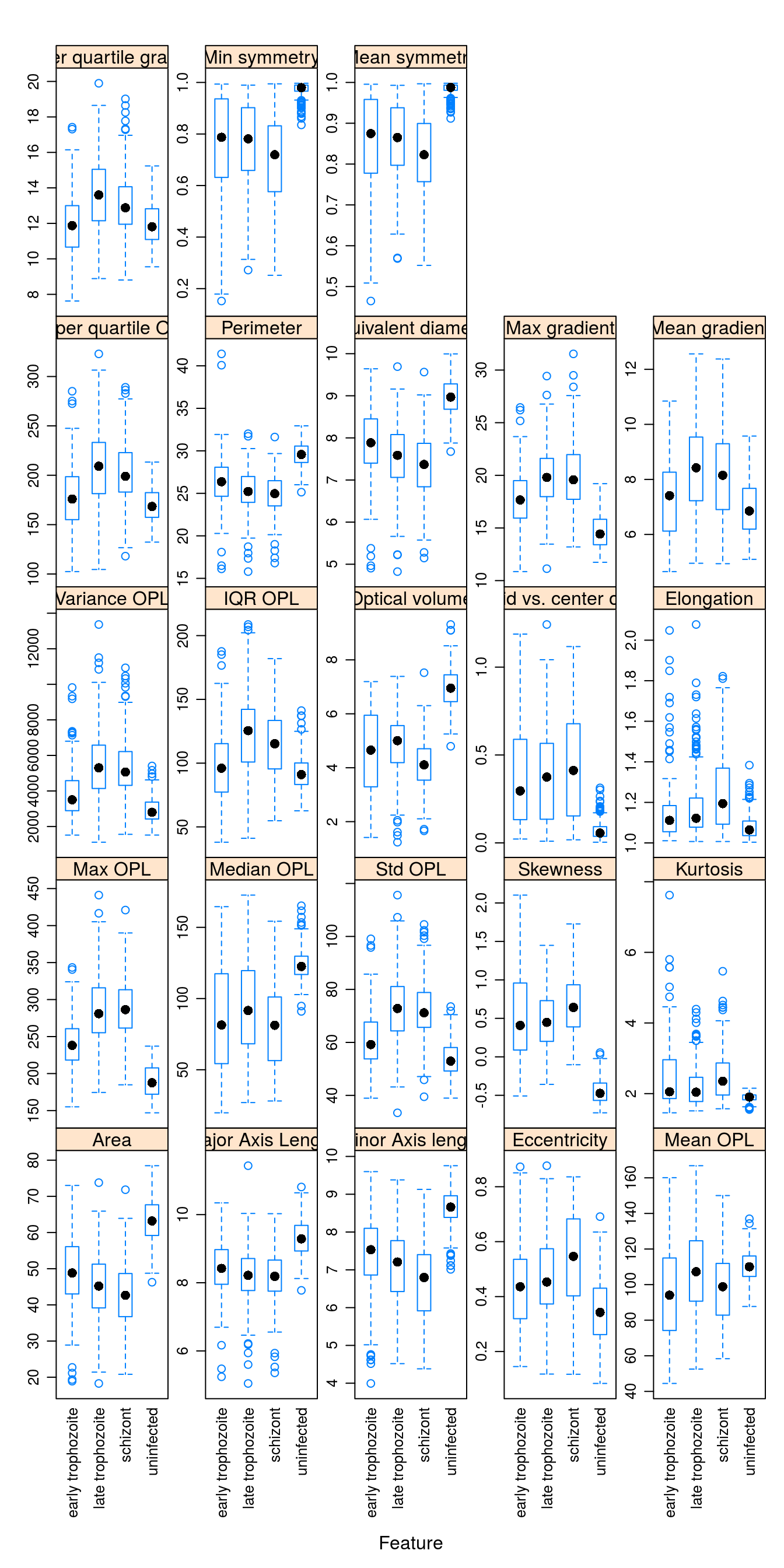 The variables in this data set are on different scales. In this situation it is important to centre and scale each predictor. A predictor variable is centered by subtracting the mean of the predictor from each value. To scale a predictor variable, each value is divided by its standard deviation. After centring and scaling the predictor variable has a mean of 0 and a standard deviation of 1.
G.2.3 Redundancy from correlated variables
Examine pairwise correlations of predictors to identify redundancy in data set
corMat <- cor(morphologyTrain)
corrplot(corMat, order="hclust", tl.cex=1)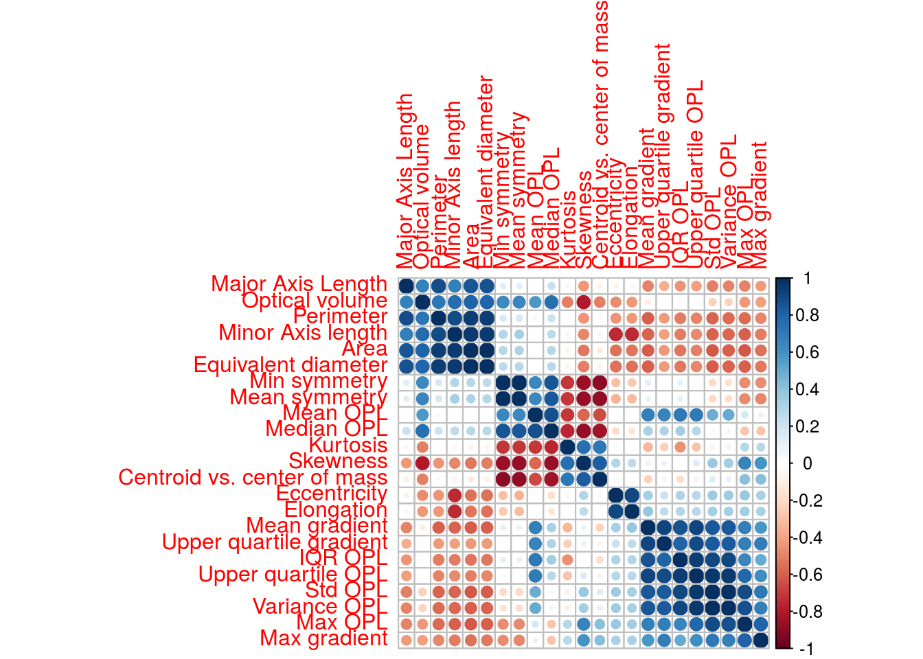
Find highly correlated predictors
highCorr <- findCorrelation(corMat, cutoff=0.75)
length(highCorr)
## [1] 16names(morphologyTrain)[highCorr]## [1] "Max OPL" "Area"
## [3] "Minor Axis length" "Std OPL"
## [5] "Equivalent diameter" "Variance OPL"
## [7] "Mean gradient" "Skewness"
## [9] "IQR OPL" "Optical volume"
## [11] "Upper quartile gradient" "Median OPL"
## [13] "Mean symmetry" "Min symmetry"
## [15] "Major Axis Length" "Elongation"G.2.4 Skewness
Observations grouped by infection status:
featurePlot(x = morphologyTrain,
            y = infectionStatusTrain,
            plot = "density",
            ## Pass in options to xyplot() to
            ## make it prettier
            scales = list(x = list(relation="free"),
                          y = list(relation="free")),
            adjust = 1.5,
            pch = "|",
            layout = c(5, 5),
            auto.key = list(columns = 2))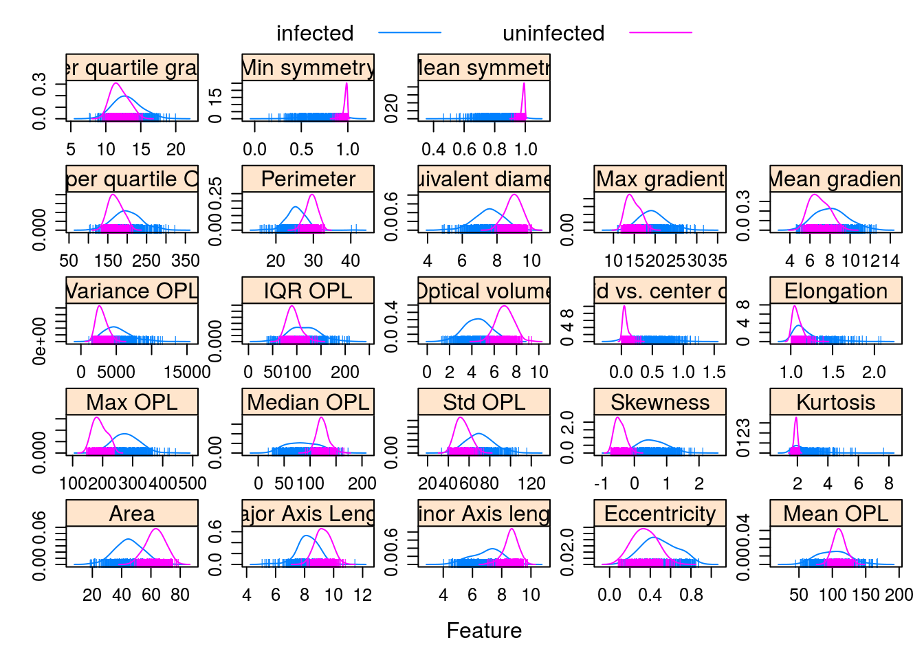
Observations grouped by infection stage:
featurePlot(x = morphologyTrain,
            y = stageTrain,
            plot = "density",
            ## Pass in options to xyplot() to
            ## make it prettier
            scales = list(x = list(relation="free"),
                          y = list(relation="free")),
            adjust = 1.5,
            pch = "|",
            layout = c(5, 5),
            auto.key = list(columns = 2))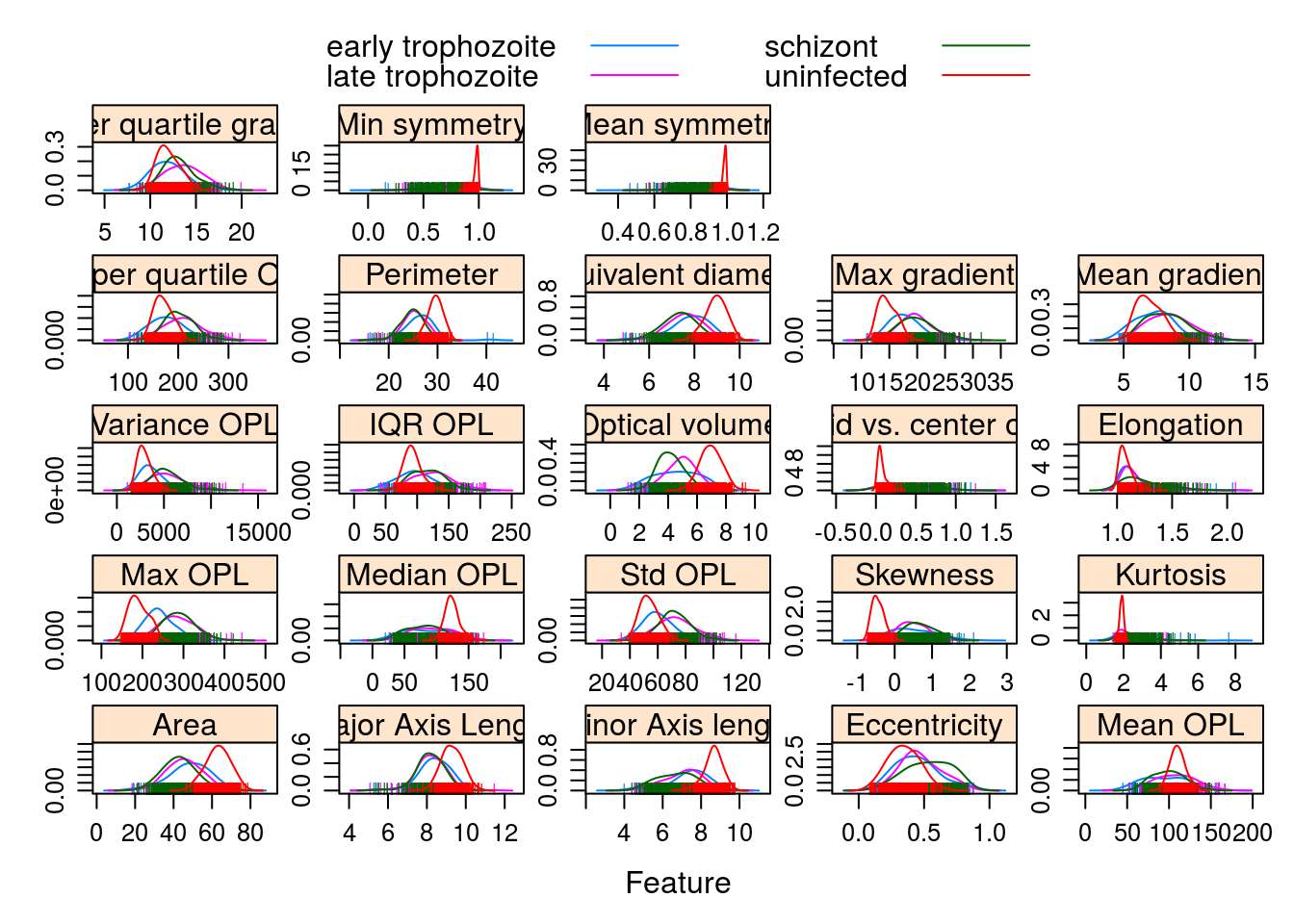
G.3 Infection status (two-class problem)
G.3.1 Model training and parameter tuning
All of the models we are going to use have a single tuning parameter. For each model we will use repeated cross validation to try 10 different values of the tuning parameter.
For each model let’s do five-fold cross-validation a total of five times. To make the analysis reproducible we need to specify the seed for each resampling iteration.
set.seed(42)
seeds <- vector(mode = "list", length = 26)
for(i in 1:25) seeds[[i]] <- sample.int(1000, 10)
seeds[[26]] <- sample.int(1000,1)

train_ctrl_infect_status <- trainControl(method="repeatedcv",
                           number = 5,
                           repeats = 5,
                           seeds = seeds,
                           summaryFunction = twoClassSummary,
                           classProbs = TRUE)
G.3.2 KNN
Train knn model:
knnFit <- train(morphologyTrain, infectionStatusTrain,
                method="knn",
                preProcess = c("center", "scale"),
                #tuneGrid=tuneParam,
                tuneLength=10,
                trControl=train_ctrl_infect_status)
## Warning in train.default(morphologyTrain, infectionStatusTrain, method =
## "knn", : The metric "Accuracy" was not in the result set. ROC will be used
## instead.knnFit## k-Nearest Neighbors
##
## 868 samples
## 23 predictors
## 2 classes: 'infected', 'uninfected'
##
## Pre-processing: centered (23), scaled (23)
## Resampling: Cross-Validated (5 fold, repeated 5 times)
## Summary of sample sizes: 695, 694, 694, 694, 695, 694, ...
## Resampling results across tuning parameters:
##
## k ROC Sens Spec
## 5 0.9956347 0.9726777 0.9937931
## 7 0.9966555 0.9692174 0.9931034
## 9 0.9967199 0.9692174 0.9931034
## 11 0.9965857 0.9702519 0.9924138
## 13 0.9963379 0.9692174 0.9910345
## 15 0.9964685 0.9678351 0.9875862
## 17 0.9966529 0.9664498 0.9882759
## 19 0.9967286 0.9661109 0.9868966
## 21 0.9970731 0.9650675 0.9868966
## 23 0.9969775 0.9654153 0.9875862
##
## ROC was used to select the optimal model using the largest value.
## The final value used for the model was k = 21.plot(knnFit)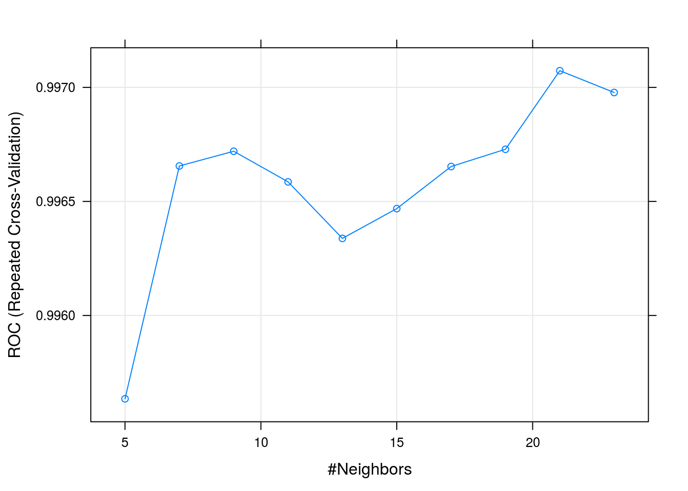
G.3.3 SVM
Train svm model:
svmFit <- train(morphologyTrain, infectionStatusTrain,
                method=svmRadialE1071,
                preProcess = c("center", "scale"),
                #tuneGrid=tuneParam,
                tuneLength=10,
                trControl=train_ctrl_infect_status)
## Warning in train.default(morphologyTrain, infectionStatusTrain, method =
## svmRadialE1071, : The metric "Accuracy" was not in the result set. ROC will
## be used instead.svmFit## Support Vector Machines with Radial Kernel - e1071
##
## 868 samples
## 23 predictors
## 2 classes: 'infected', 'uninfected'
##
## Pre-processing: centered (23), scaled (23)
## Resampling: Cross-Validated (5 fold, repeated 5 times)
## Summary of sample sizes: 694, 694, 695, 694, 695, 694, ...
## Resampling results across tuning parameters:
##
## cost ROC Sens Spec
## 0.25 0.9977719 0.9764948 0.9848276
## 0.50 0.9979155 0.9806417 0.9931034
## 1.00 0.9980584 0.9813343 0.9917241
## 2.00 0.9983201 0.9820270 0.9931034
## 4.00 0.9983314 0.9813343 0.9931034
## 8.00 0.9981986 0.9827226 0.9931034
## 16.00 0.9982936 0.9847886 0.9931034
## 32.00 0.9980604 0.9851334 0.9889655
## 64.00 0.9974875 0.9837481 0.9882759
## 128.00 0.9970936 0.9823688 0.9841379
##
## ROC was used to select the optimal model using the largest value.
## The final value used for the model was cost = 4.plot(svmFit, scales = list(x = list(log =2)))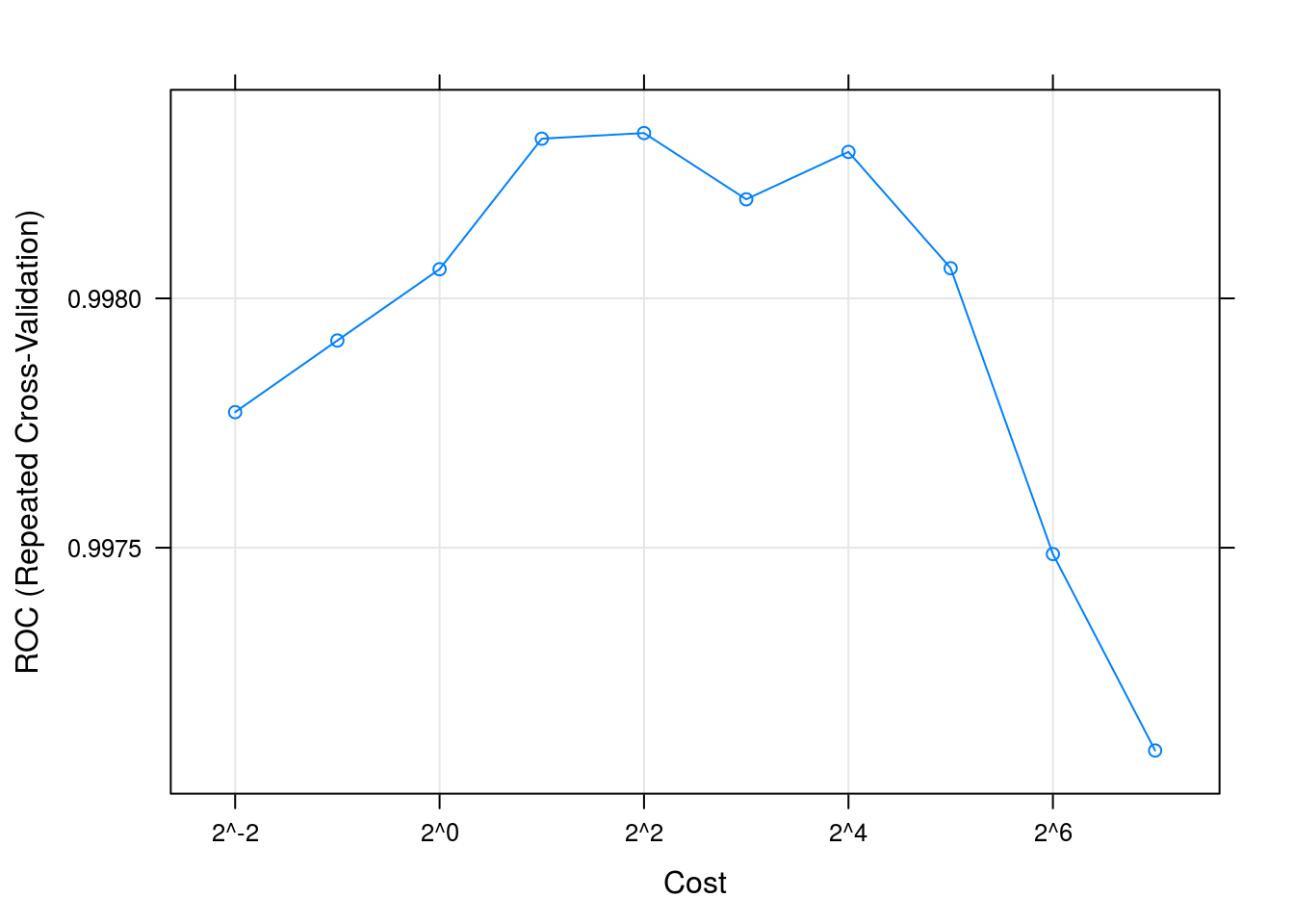
G.3.4 Decision tree
Train decision tree model:
dtFit <- train(morphologyTrain, infectionStatusTrain,
                method="rpart",
                preProcess = c("center", "scale"),
                #tuneGrid=tuneParam,
                tuneLength=10,
                trControl=train_ctrl_infect_status)
## Warning in train.default(morphologyTrain, infectionStatusTrain, method =
## "rpart", : The metric "Accuracy" was not in the result set. ROC will be
## used instead.dtFit## CART
##
## 868 samples
## 23 predictors
## 2 classes: 'infected', 'uninfected'
##
## Pre-processing: centered (23), scaled (23)
## Resampling: Cross-Validated (5 fold, repeated 5 times)
## Summary of sample sizes: 694, 695, 694, 695, 694, 694, ...
## Resampling results across tuning parameters:
##
## cp ROC Sens Spec
## 0.00000000 0.9752903 0.9754423 0.9634483
## 0.09885057 0.9523538 0.9619490 0.9427586
## 0.19770115 0.9523538 0.9619490 0.9427586
## 0.29655172 0.9523538 0.9619490 0.9427586
## 0.39540230 0.9523538 0.9619490 0.9427586
## 0.49425287 0.9523538 0.9619490 0.9427586
## 0.59310345 0.9523538 0.9619490 0.9427586
## 0.69195402 0.9523538 0.9619490 0.9427586
## 0.79080460 0.9523538 0.9619490 0.9427586
## 0.88965517 0.8015262 0.9733973 0.6296552
##
## ROC was used to select the optimal model using the largest value.
## The final value used for the model was cp = 0.plot(dtFit)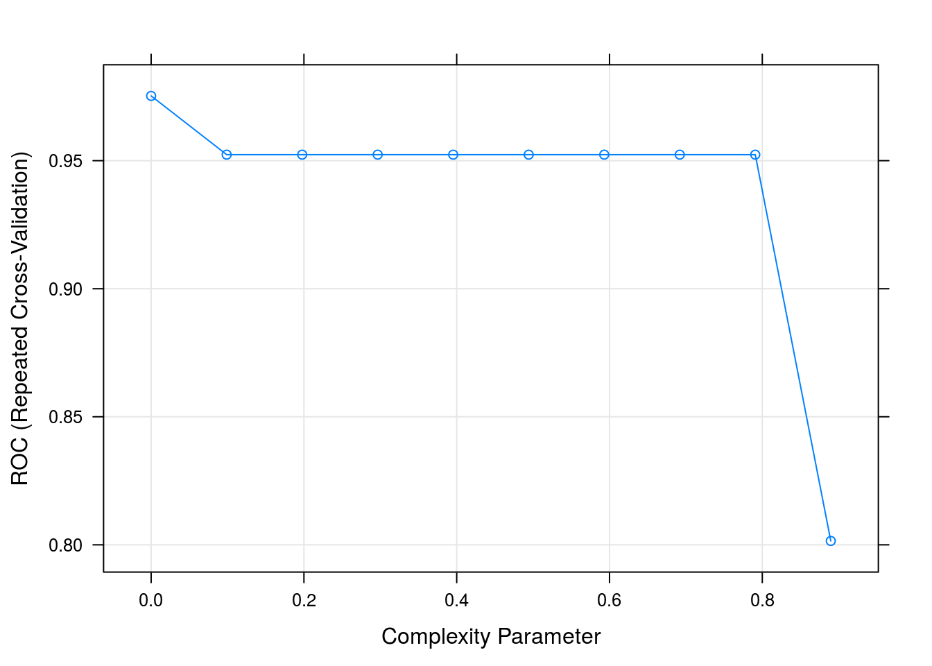
prp(dtFit$finalModel)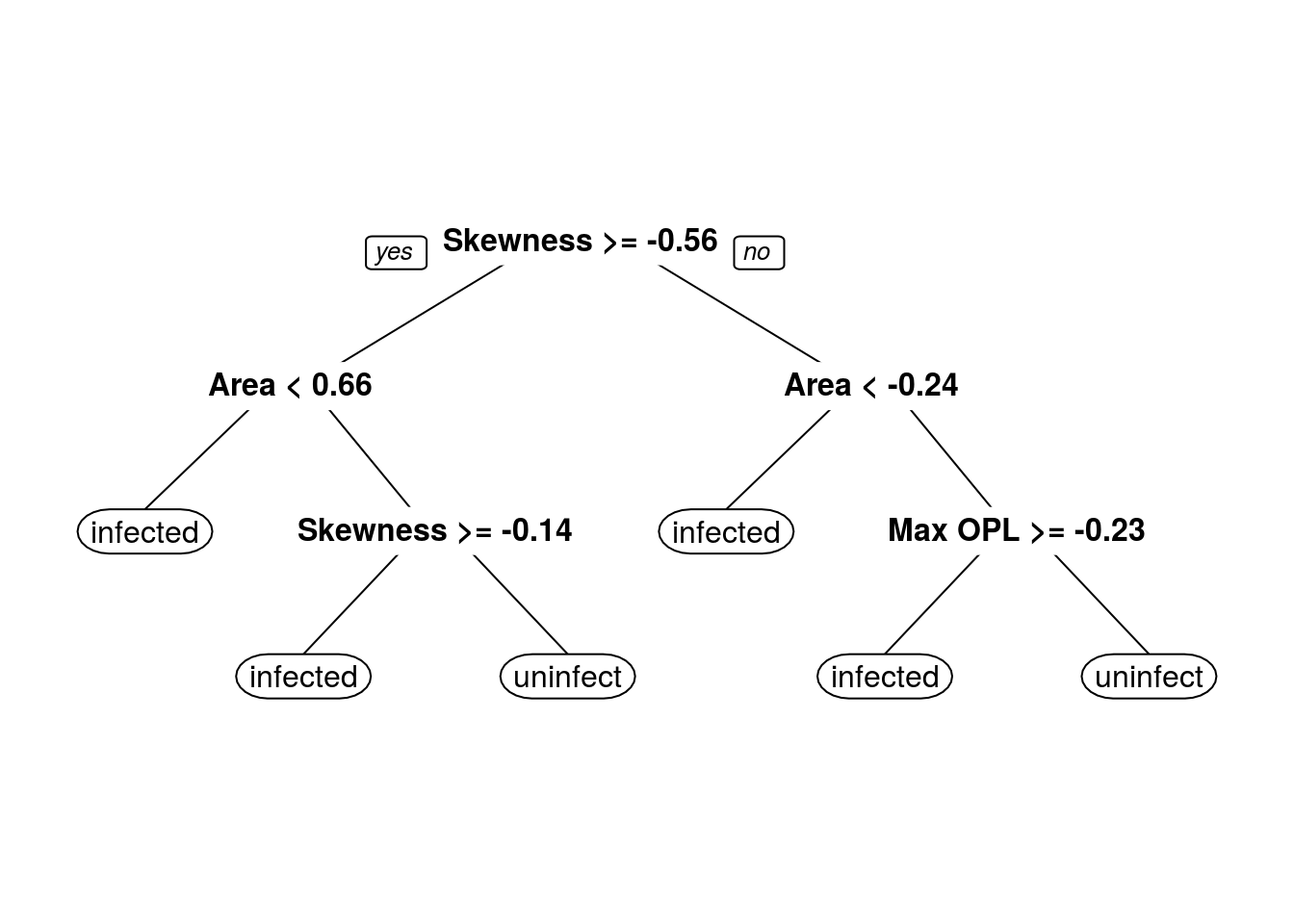
G.3.5 Random forest
rfFit <- train(morphologyTrain, infectionStatusTrain,
                method="rf",
                preProcess = c("center", "scale"),
                #tuneGrid=tuneParam,
                tuneLength=10,
                trControl=train_ctrl_infect_status)
## Warning in train.default(morphologyTrain, infectionStatusTrain, method =
## "rf", : The metric "Accuracy" was not in the result set. ROC will be used
## instead.rfFit## Random Forest
##
## 868 samples
## 23 predictors
## 2 classes: 'infected', 'uninfected'
##
## Pre-processing: centered (23), scaled (23)
## Resampling: Cross-Validated (5 fold, repeated 5 times)
## Summary of sample sizes: 694, 694, 695, 694, 695, 694, ...
## Resampling results across tuning parameters:
##
## mtry ROC Sens Spec
## 2 0.9981532 0.9868666 0.9813793
## 4 0.9979057 0.9879010 0.9868966
## 6 0.9977327 0.9885937 0.9855172
## 9 0.9973191 0.9892834 0.9841379
## 11 0.9973216 0.9892834 0.9820690
## 13 0.9967486 0.9889355 0.9813793
## 16 0.9968264 0.9882399 0.9793103
## 18 0.9964275 0.9878921 0.9772414
## 20 0.9959667 0.9875442 0.9772414
## 23 0.9941175 0.9868516 0.9765517
##
## ROC was used to select the optimal model using the largest value.
## The final value used for the model was mtry = 2.plot(rfFit)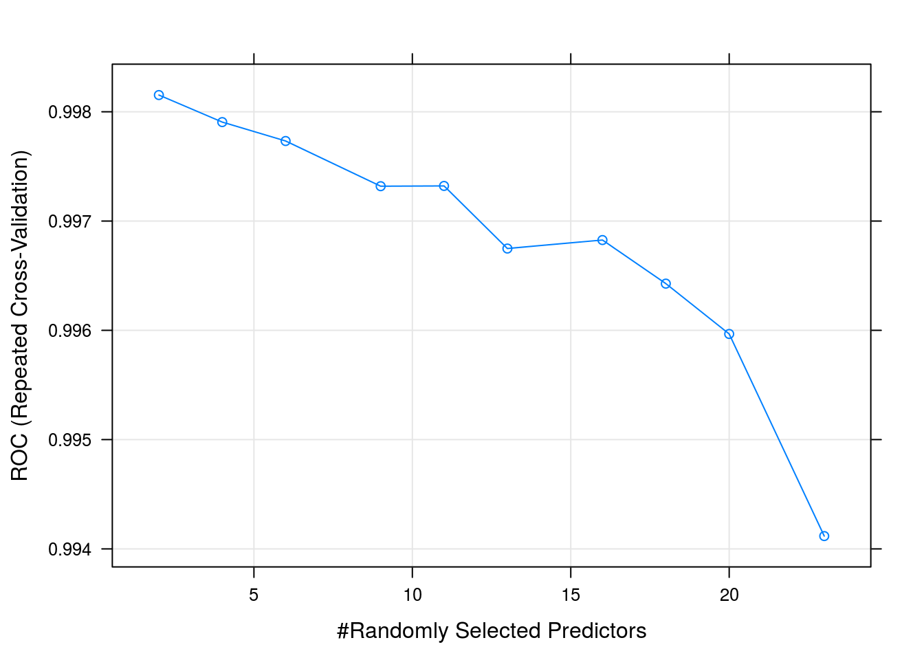
G.3.6 Compare models
Make a list of our models
model_list <- list(knn=knnFit,
                   svm=svmFit,
                   decisionTree=dtFit,
                   randomForest=rfFit)
Collect resampling results for each model
resamps <- resamples(model_list)
resamps
##
## Call:
## resamples.default(x = model_list)
##
## Models: knn, svm, decisionTree, randomForest
## Number of resamples: 25
## Performance metrics: ROC, Sens, Spec
## Time estimates for: everything, final model fitsummary(resamps)##
## Call:
## summary.resamples(object = resamps)
##
## Models: knn, svm, decisionTree, randomForest
## Number of resamples: 25
##
## ROC
## Min. 1st Qu. Median Mean 3rd Qu. Max.
## knn 0.9925684 0.9952774 0.9980510 0.9970731 0.9985880 0.9998501
## svm 0.9933115 0.9965815 0.9995541 0.9983314 1.0000000 1.0000000
## decisionTree 0.9357907 0.9716855 0.9778537 0.9752903 0.9826087 0.9976962
## randomForest 0.9939061 0.9971514 0.9994003 0.9981532 0.9997027 1.0000000
## NA's
## knn 0
## svm 0
## decisionTree 0
## randomForest 0
##
## Sens
## Min. 1st Qu. Median Mean 3rd Qu. Max. NA's
## knn 0.9224138 0.9565217 0.9655172 0.9650675 0.9826087 1 0
## svm 0.9482759 0.9741379 0.9827586 0.9813343 0.9913043 1 0
## decisionTree 0.9217391 0.9655172 0.9741379 0.9754423 0.9827586 1 0
## randomForest 0.9568966 0.9826087 0.9913043 0.9868666 1.0000000 1 0
##
## Spec
## Min. 1st Qu. Median Mean 3rd Qu. Max. NA's
## knn 0.9482759 0.9827586 0.9827586 0.9868966 1.0000000 1 0
## svm 0.9827586 0.9827586 1.0000000 0.9931034 1.0000000 1 0
## decisionTree 0.8793103 0.9482759 0.9827586 0.9634483 0.9827586 1 0
## randomForest 0.9310345 0.9827586 0.9827586 0.9813793 1.0000000 1 0bwplot(resamps)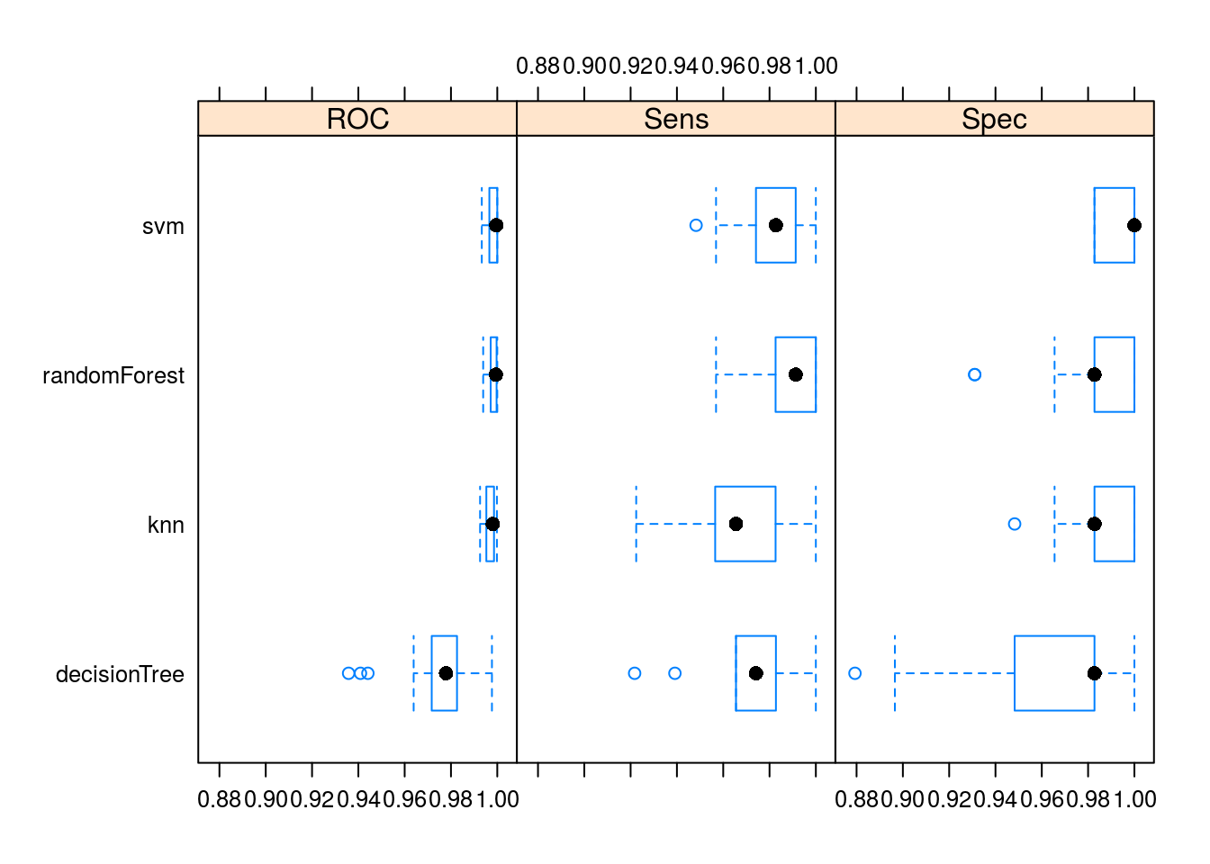
G.3.7 Predict test set using our best model
test_pred <- predict(svmFit, morphologyTest)
confusionMatrix(test_pred, infectionStatusTest)
## Confusion Matrix and Statistics
##
## Reference
## Prediction infected uninfected
## infected 242 3
## uninfected 4 120
##
## Accuracy : 0.981
## 95% CI : (0.9613, 0.9923)
## No Information Rate : 0.6667
## P-Value [Acc > NIR] : <2e-16
##
## Kappa : 0.9574
## Mcnemar's Test P-Value : 1
##
## Sensitivity : 0.9837
## Specificity : 0.9756
## Pos Pred Value : 0.9878
## Neg Pred Value : 0.9677
## Prevalence : 0.6667
## Detection Rate : 0.6558
## Detection Prevalence : 0.6640
## Balanced Accuracy : 0.9797
##
## 'Positive' Class : infected
## G.3.8 ROC curve
svmProbs <- predict(svmFit, morphologyTest, type="prob")
head(svmProbs)
## infected uninfected
## normal_..4 0.019842960 0.98015704
## normal_..7 0.959900420 0.04009958
## normal_.12 0.009452970 0.99054703
## normal_.17 0.002097783 0.99790222
## normal_.18 0.003581587 0.99641841
## normal_.19 0.024682569 0.97531743svmROC <- roc(infectionStatusTest, svmProbs[,"infected"])
auc(svmROC)## Area under the curve: 0.9977plot(svmROC)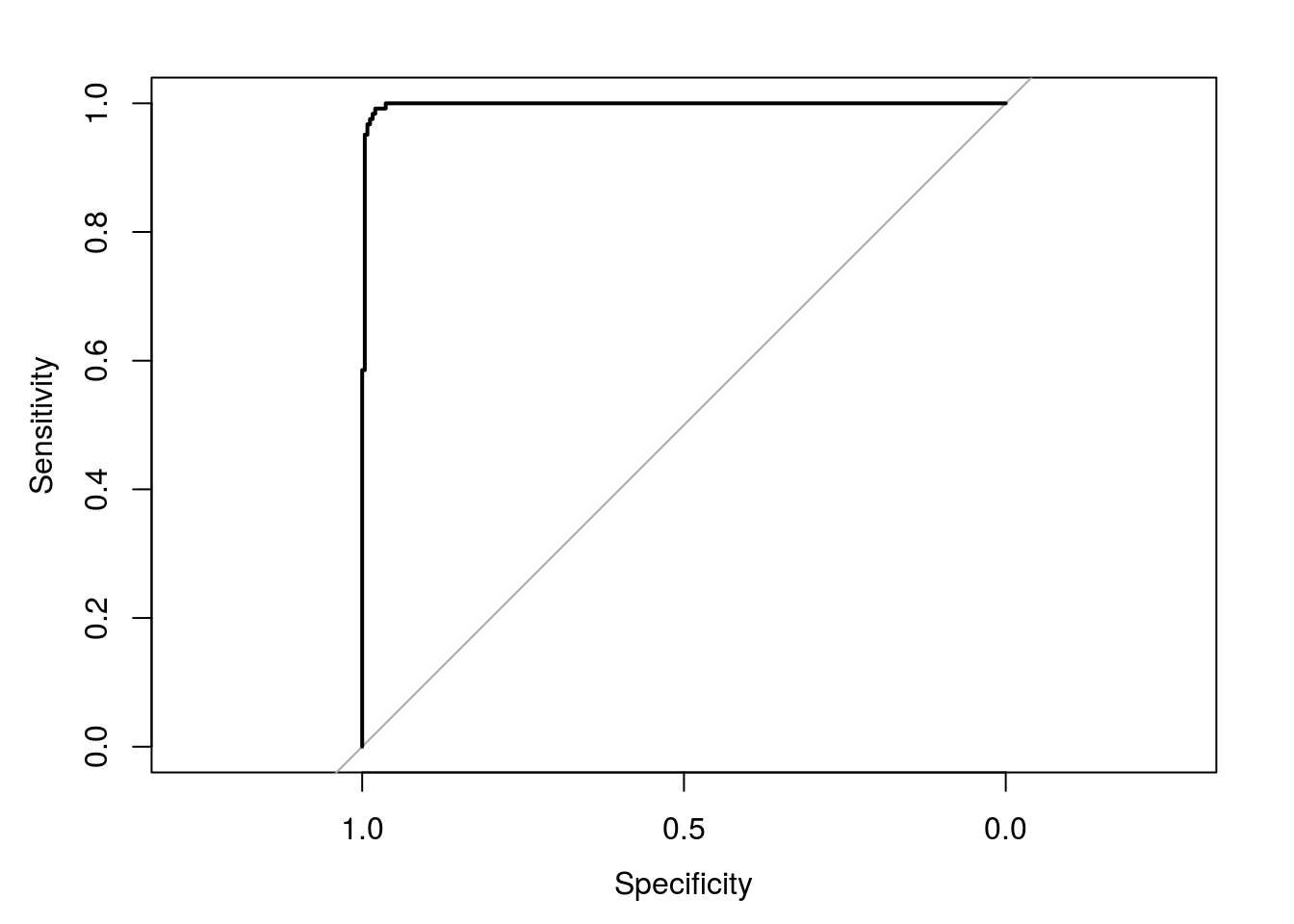
G.4 Discrimination of infective stages (multi-class problem)
G.4.1 Define cross-validation procedure
train_ctrl_stage <- trainControl(method="repeatedcv",
                           number = 5,
                           repeats = 5,
                           seeds = seeds)
G.4.2 KNN
Train knn model with all variables:
knnFit <- train(morphologyTrain, stageTrain,
                method="knn",
                preProcess = c("center", "scale"),
                #tuneGrid=tuneParam,
                tuneLength=10,
                trControl=train_ctrl_stage)

knnFit
## k-Nearest Neighbors
##
## 868 samples
## 23 predictors
## 4 classes: 'early trophozoite', 'late trophozoite', 'schizont', 'uninfected'
##
## Pre-processing: centered (23), scaled (23)
## Resampling: Cross-Validated (5 fold, repeated 5 times)
## Summary of sample sizes: 694, 695, 693, 695, 695, 695, ...
## Resampling results across tuning parameters:
##
## k Accuracy Kappa
## 5 0.6806513 0.5576508
## 7 0.6940101 0.5754335
## 9 0.6949123 0.5762065
## 11 0.6931076 0.5731317
## 13 0.6940246 0.5743092
## 15 0.6917084 0.5706892
## 17 0.6917110 0.5704146
## 19 0.6958385 0.5759926
## 21 0.6956085 0.5755366
## 23 0.6958385 0.5755180
##
## Accuracy was used to select the optimal model using the largest value.
## The final value used for the model was k = 19.plot(knnFit)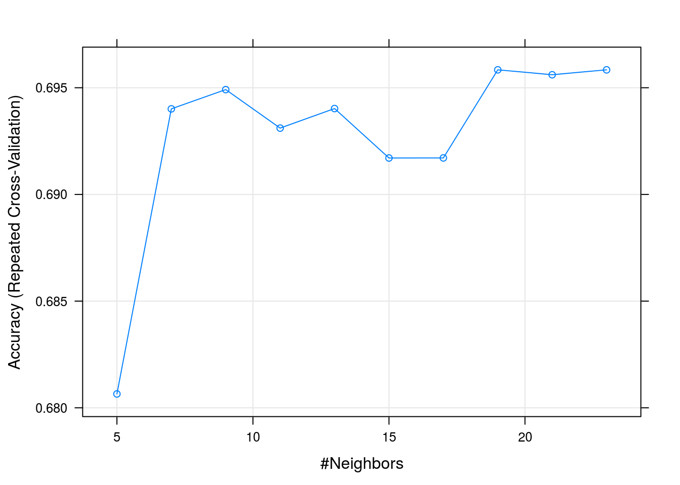
G.4.3 SVM
Train SVM model with all variables:
svmFit <- train(morphologyTrain, stageTrain,
                method=svmRadialE1071,
                preProcess = c("center", "scale"),
                #tuneGrid=tuneParam,
                tuneLength=10,
                trControl=train_ctrl_stage)

svmFit
## Support Vector Machines with Radial Kernel - e1071
##
## 868 samples
## 23 predictors
## 4 classes: 'early trophozoite', 'late trophozoite', 'schizont', 'uninfected'
##
## Pre-processing: centered (23), scaled (23)
## Resampling: Cross-Validated (5 fold, repeated 5 times)
## Summary of sample sizes: 693, 695, 695, 694, 695, 694, ...
## Resampling results across tuning parameters:
##
## cost Accuracy Kappa
## 0.25 0.7078501 0.5940116
## 0.50 0.7156902 0.6063755
## 1.00 0.7195864 0.6124250
## 2.00 0.7198083 0.6134929
## 4.00 0.7198030 0.6136120
## 8.00 0.7207491 0.6154010
## 16.00 0.7138537 0.6068131
## 32.00 0.6991156 0.5874694
## 64.00 0.6869050 0.5717486
## 128.00 0.6763009 0.5579433
##
## Accuracy was used to select the optimal model using the largest value.
## The final value used for the model was cost = 8.plot(svmFit, scales = list(x = list(log =2)))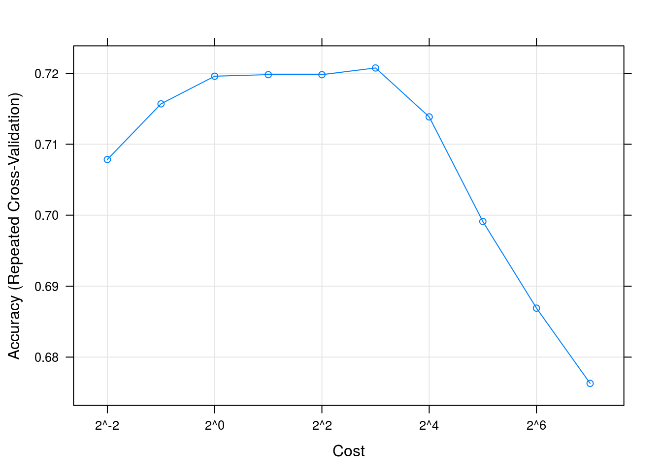
G.4.4 Decision tree
Train decision tree model with all variables:
dtFit <- train(morphologyTrain, stageTrain,
                method="rpart",
                preProcess = c("center", "scale"),
                #tuneGrid=tuneParam,
                tuneLength=10,
                trControl=train_ctrl_stage)

dtFit
## CART
##
## 868 samples
## 23 predictors
## 4 classes: 'early trophozoite', 'late trophozoite', 'schizont', 'uninfected'
##
## Pre-processing: centered (23), scaled (23)
## Resampling: Cross-Validated (5 fold, repeated 5 times)
## Summary of sample sizes: 693, 695, 695, 694, 695, 694, ...
## Resampling results across tuning parameters:
##
## cp Accuracy Kappa
## 0.005190311 0.6850209 0.5667306
## 0.006920415 0.6864227 0.5691875
## 0.007785467 0.6871071 0.5706621
## 0.010380623 0.6799831 0.5607537
## 0.012110727 0.6825278 0.5637137
## 0.013840830 0.6815977 0.5624175
## 0.015570934 0.6811498 0.5609683
## 0.034602076 0.6820522 0.5613656
## 0.124567474 0.6184755 0.4610759
## 0.399653979 0.3964157 0.1019836
##
## Accuracy was used to select the optimal model using the largest value.
## The final value used for the model was cp = 0.007785467.plot(dtFit)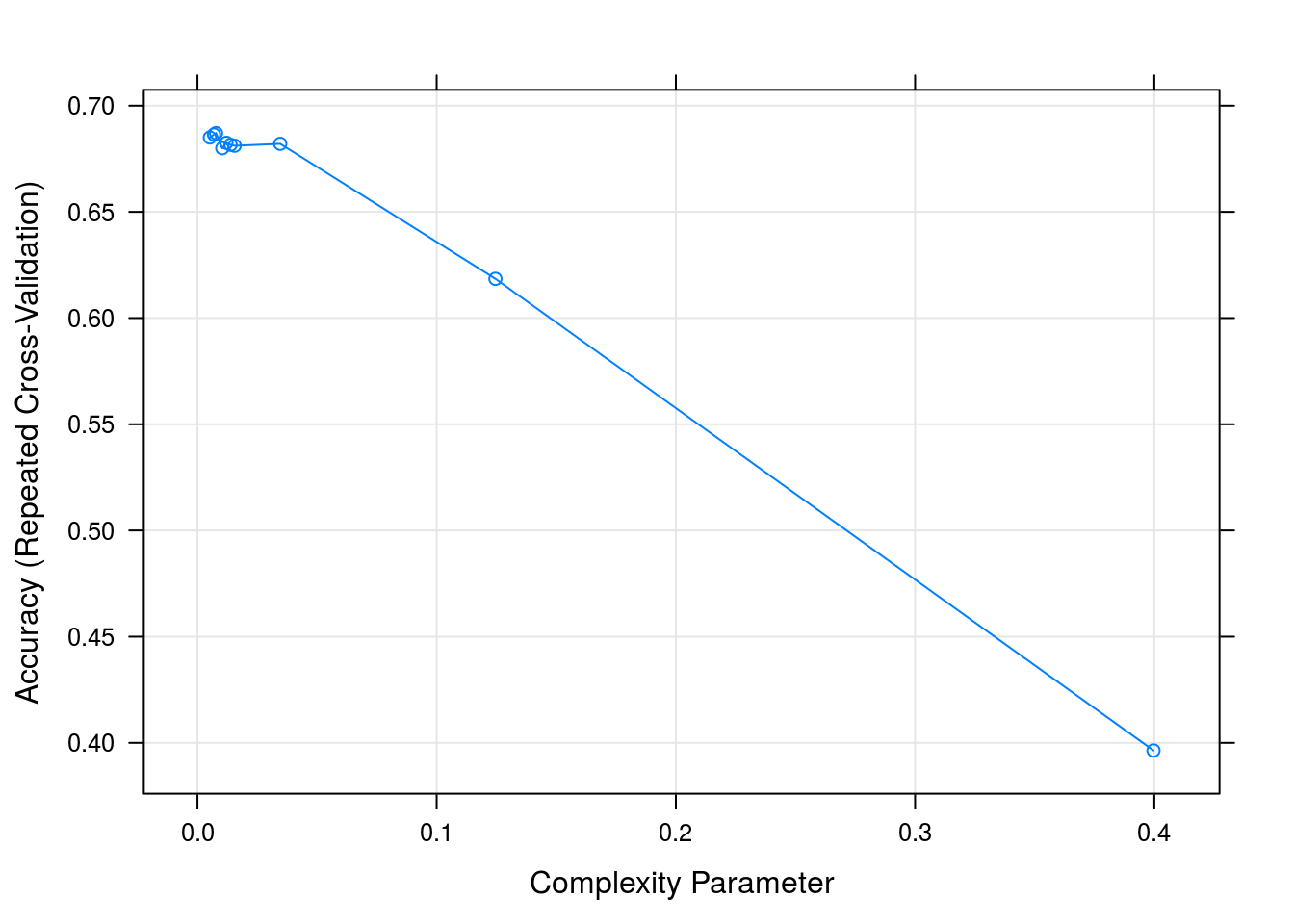
prp(dtFit$finalModel)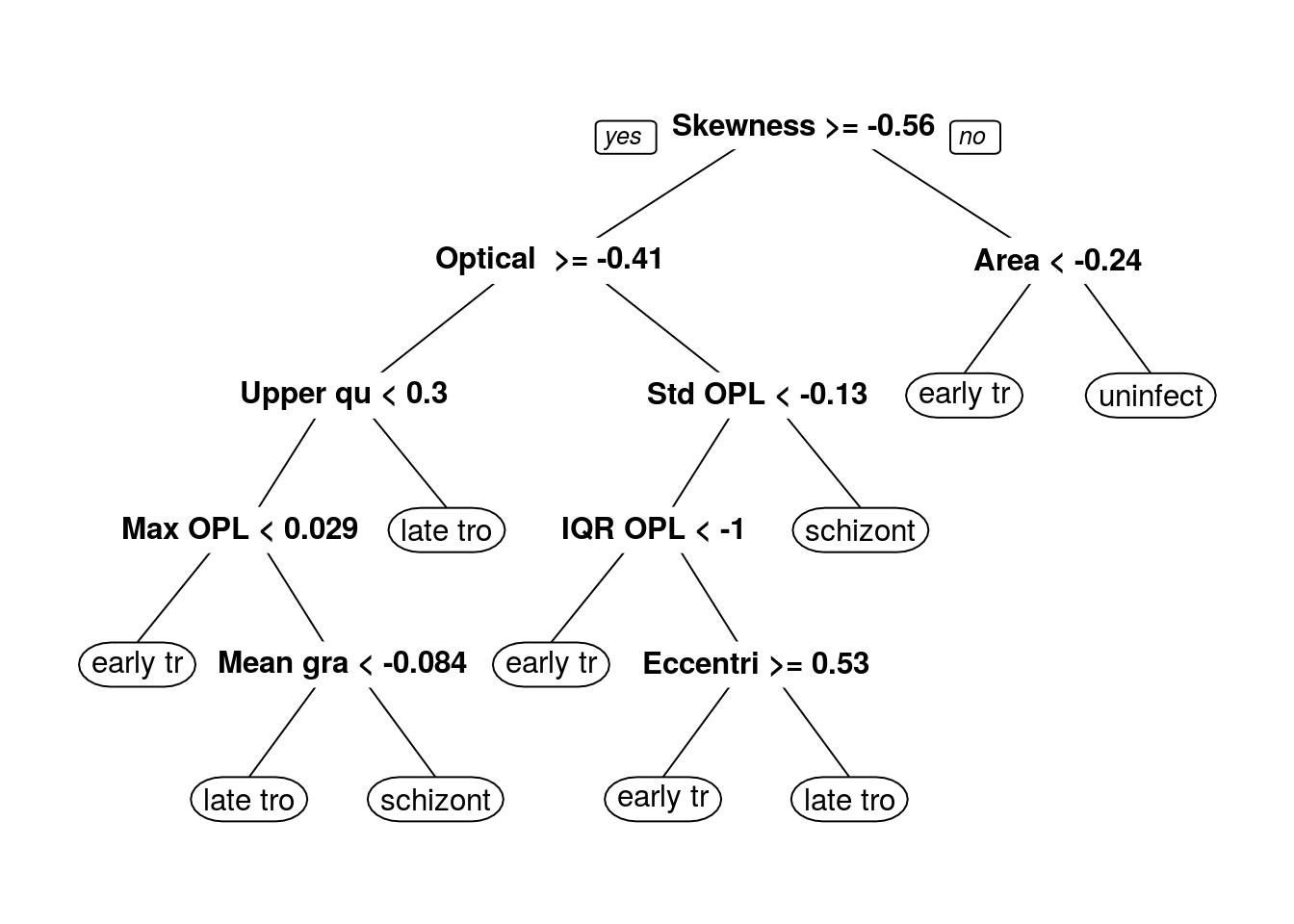
G.4.5 Random forest
Train random forest model with all variables:
rfFit <- train(morphologyTrain, stageTrain,
                method="rf",
                preProcess = c("center", "scale"),
                #tuneGrid=tuneParam,
                tuneLength=10,
                trControl=train_ctrl_stage)

rfFit
## Random Forest
##
## 868 samples
## 23 predictors
## 4 classes: 'early trophozoite', 'late trophozoite', 'schizont', 'uninfected'
##
## Pre-processing: centered (23), scaled (23)
## Resampling: Cross-Validated (5 fold, repeated 5 times)
## Summary of sample sizes: 693, 695, 695, 694, 695, 694, ...
## Resampling results across tuning parameters:
##
## mtry Accuracy Kappa
## 2 0.7184462 0.6121623
## 4 0.7179838 0.6120214
## 6 0.7232845 0.6196398
## 9 0.7248884 0.6221363
## 11 0.7209591 0.6167334
## 13 0.7230175 0.6196534
## 16 0.7195890 0.6150192
## 18 0.7181885 0.6132322
## 20 0.7184422 0.6133707
## 23 0.7149754 0.6086754
##
## Accuracy was used to select the optimal model using the largest value.
## The final value used for the model was mtry = 9.plot(rfFit)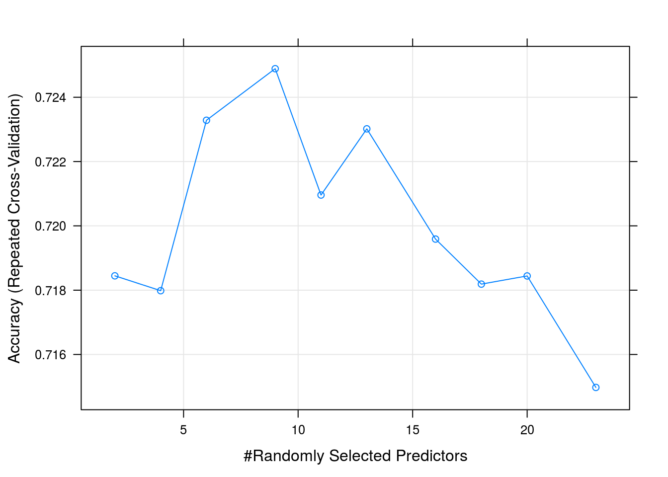
G.4.6 Compare models
Make a list of our models
model_list <- list(knn=knnFit,
                   svm=svmFit,
                   decisionTree=dtFit,
                   randomForest=rfFit)
Collect resampling results for each model
resamps <- resamples(model_list)
resamps
##
## Call:
## resamples.default(x = model_list)
##
## Models: knn, svm, decisionTree, randomForest
## Number of resamples: 25
## Performance metrics: Accuracy, Kappa
## Time estimates for: everything, final model fitsummary(resamps)##
## Call:
## summary.resamples(object = resamps)
##
## Models: knn, svm, decisionTree, randomForest
## Number of resamples: 25
##
## Accuracy
## Min. 1st Qu. Median Mean 3rd Qu. Max.
## knn 0.6494253 0.6763006 0.6896552 0.6958385 0.7142857 0.7643678
## svm 0.6666667 0.6994220 0.7241379 0.7207491 0.7341040 0.7873563
## decisionTree 0.6494253 0.6647399 0.6820809 0.6871071 0.7011494 0.7514451
## randomForest 0.6820809 0.7109827 0.7225434 0.7248884 0.7413793 0.7745665
## NA's
## knn 0
## svm 0
## decisionTree 0
## randomForest 0
##
## Kappa
## Min. 1st Qu. Median Mean 3rd Qu. Max.
## knn 0.5132532 0.5494582 0.5659846 0.5759926 0.6029405 0.6719246
## svm 0.5396405 0.5873584 0.6199144 0.6154010 0.6334746 0.7079477
## decisionTree 0.5204446 0.5381140 0.5650286 0.5706621 0.5876401 0.6588554
## randomForest 0.5631113 0.6014192 0.6164257 0.6221363 0.6424494 0.6931089
## NA's
## knn 0
## svm 0
## decisionTree 0
## randomForest 0bwplot(resamps)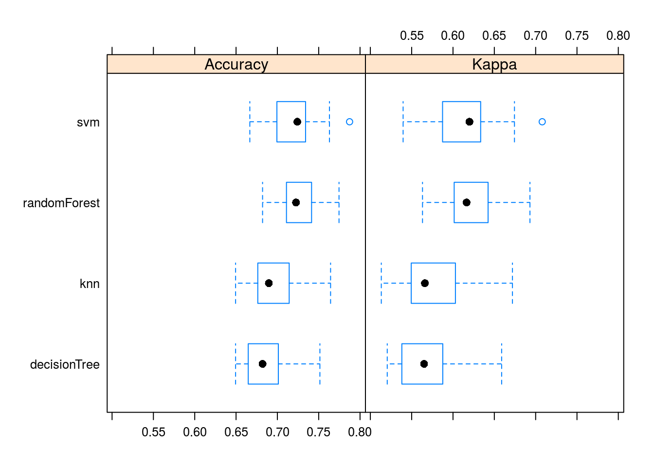
G.4.7 Predict test set using our best model
test_pred <- predict(rfFit, morphologyTest)
confusionMatrix(test_pred, stageTest)
## Confusion Matrix and Statistics
##
## Reference
## Prediction early trophozoite late trophozoite schizont uninfected
## early trophozoite 27 3 7 3
## late trophozoite 16 57 28 0
## schizont 5 33 66 0
## uninfected 3 1 0 120
##
## Overall Statistics
##
## Accuracy : 0.7317
## 95% CI : (0.6834, 0.7763)
## No Information Rate : 0.3333
## P-Value [Acc > NIR] : < 2.2e-16
##
## Kappa : 0.6305
## Mcnemar's Test P-Value : NA
##
## Statistics by Class:
##
## Class: early trophozoite Class: late trophozoite
## Sensitivity 0.52941 0.6064
## Specificity 0.95912 0.8400
## Pos Pred Value 0.67500 0.5644
## Neg Pred Value 0.92705 0.8619
## Prevalence 0.13821 0.2547
## Detection Rate 0.07317 0.1545
## Detection Prevalence 0.10840 0.2737
## Balanced Accuracy 0.74427 0.7232
## Class: schizont Class: uninfected
## Sensitivity 0.6535 0.9756
## Specificity 0.8582 0.9837
## Pos Pred Value 0.6346 0.9677
## Neg Pred Value 0.8679 0.9878
## Prevalence 0.2737 0.3333
## Detection Rate 0.1789 0.3252
## Detection Prevalence 0.2818 0.3360
## Balanced Accuracy 0.7558 0.9797